Noise

Notes from the book “Noise is Beautiful”.

Generating Randomness §

True randomness is difficult to generate. Instead, we often will generate pseudo-random numbers, deterministic algorithms that generate numbers that look random.

In this section, we describe various ways we can generate these pseudo-random numbers.

Integer Hash §

Classical random number generators typically use a single integer as a seed, which can be set when calling the function. They then use this seed to apply a fixed number of operations on the input to generate a “random” number.

One example of this is the Permuted Congruential Generator (PCG) Hash, originally presented by Melissa O’Neill in 2014. This is an integer hash that is widely used in computer graphics.

uint pcg_hash(uint input) {
    uint state = input * 747796405u + 2891336453u;
    uint word = ((state >> ((state >> 28u) + 4u)) ^ state) * 277803737u;
    return (word >> 22u) ^ word;
}

This hash works on a 1-dimensional input, but can be generalized to accept higher-dimensional input by chaining hash function calls on the input parameters

hash(x,y) = hash(hash(x) + y)

One example is as follows:

flag cellnoise_pcg2(vec2 p) {
    // Convert to integer input, and apply a bit mask to remove the 
    // sign bit
    uvec2 pu = uvec2(ivec2(floor(p)) & ivec2(0x7FFFFFFF));
    // Chain hash calls and then squish the noise output to [0,1]
    return float(pcg_hash(pu.x + pcg_hash(pu.y)) & 0xFFFFu) / 65536.0;
}

Floating Point Hashes §

While the above hash works well, integers are often not very well supported on GPUs. In many cases, integer math can have lower performance than floating point math on GPUs. Because of this, we also need to discuss hash functions that also work on floating point inputs.

Permutation Polynomials §

One algorithm that works well is a permutation polynomial. These are polynomials that permute a sequence of consequtive integers $\{0,1,2,3,\dots N-1\}$.

Interestingly, quadratic polynomials of the form

$$p(x)=(2A{x}^2+Bx)\mathrm{mod}{A}^2$$

For prime $A$ are guaranteed to be permutation polynomials. This gives us well-distributed output values if the input values are also evenly distributed.

One example of this function is $p(x)=(34x^2+10x)\mathrm{mod}289$ ($A=17,B=10$).

float permute(float x) {
    float h = mod(x, 289.0f);
    return mod((34.0 * h + 10.0) * h, 289.0);
}
 
// As always, we can generalize this to higher dimensions by chaining
float cellnoise_perm(vec2 p) {
    // The division by 288.0 normalizes to [0,1].
    return permute(permute(p.x) + p.y) / 288.0;
}

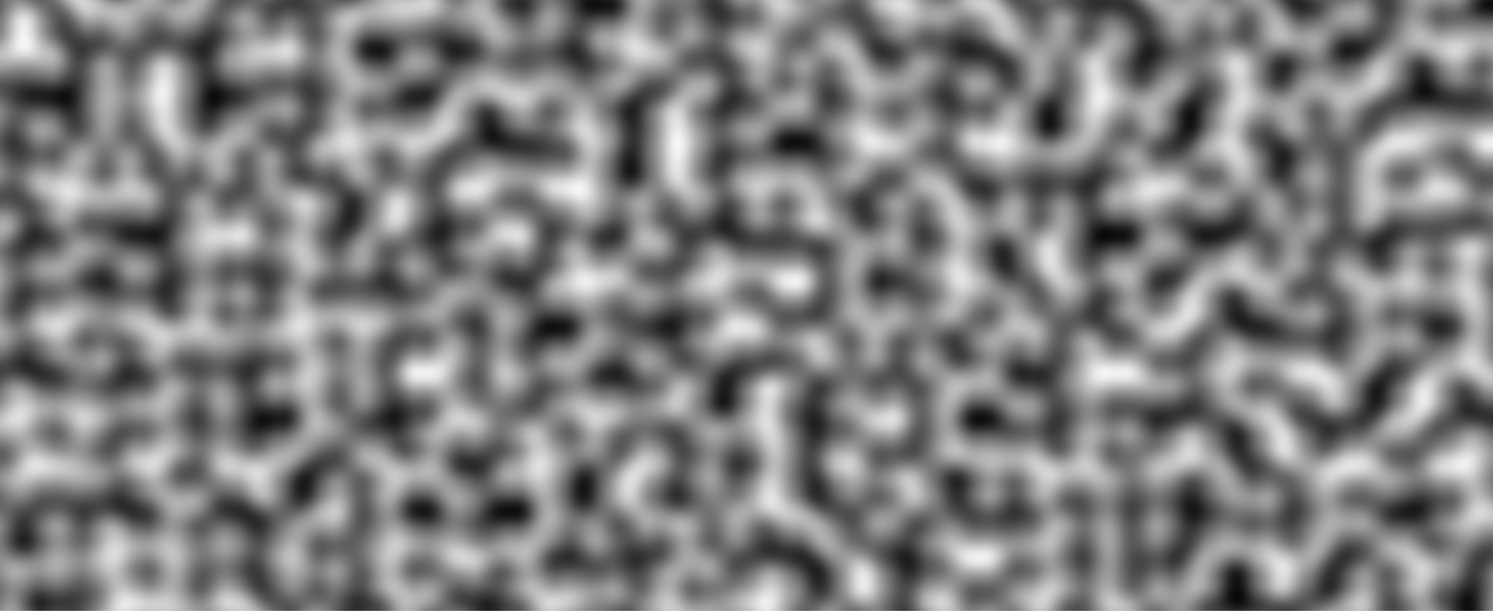
Permute289, Sample Output

Sample output generated by ShaderToy

Trash Bits §

Another method, albeit a bit of a hack, is by using imprecision in the sin function.

float cellnoise_sin(vec2 p) {
    return fract(sin(dot(p, vec2(12.9898, 78.233))) * 43758.5453);
}

When scaled to to large values, bit imprecision makes sin generate values that appear random. So, we turn out 2D vector into a 1D input using values that probably don’t cause artifacts, and only take the fractional part of the scaled output.

This is a hack that is not recommended to be used, as it abuses imprecision in the sin function which is undocumented for this scale.

Trash Bits, Sample Output

Sample output generated by ShaderToy

Ad-Hoc Float Hash §

Finally, we have a methjod suggested by Dave Hoskins on Shadertoy, which uses the fract function. This method is similar to the use of sin above, but doesn’t use the imprecision of sin.

float hash12(vec2 p) {
    vec3 p3 = fract(vec3(p.xyx) * 0.1031);
    p3 += dot(p3, p3.yzx + 33.33);
    return fract((p3.x + p3.y) * p3.z);
}

Dave's Method, Sample Output

Sample output generated by ShaderToy

This method generates pretty good results!

Perlin Noise §

In many cases, we want randomness, but randomness that has an inherent pattern to it. This “random pattern” can then be used to add smaller details to our objects, at (relatively) cheap costs.

The defacto standard for doing generating this noise is Perlin Noise, first proposed by Ken Perlin in 1985.

Effects like this can also be generated by summing sine waves, but Perlin Noise achieves the same effect in significantly less computations.

Generating Noise (2D) §

Perlin noise works as follows:

• On a regular grid, generate random gradient vectors at each point.
• For any point, find the gradient vectors of the grid cell it’s in, and interpolate between the gradient vectors to find the noise value.

Let’s consider the 2D case. The algorithm is as follows:

1. Assign pseudo-random gradients to each point in the grid, and a function value of 0.
2. For a point $p$ on the grid, find $s,t$, where in the cell the point is, by taking $p$’s fractional component.
   • $s=fract(p.x),t=fract(p.y)$.
3. Find $v_{00},v_{10},v_{01},v_{11}$, the directional vectors from the cell’s corner to $p$.
   • The binary in the subscript denotes what corner we’re talking about. $v_{00}$ is the bottom-left corner, and $v_{11}$ is the top-right corner.
4. Find $n_{ij}=g_{ij}\cdot v_{ij}$, the “influence” the gradient has at that point.
5. Interpolate between each of our $n_{ij}^{\prime }s$ to find the value at our point, first along one dimension (say x), then the next (say y).
   • Before interpolating, we first apply a blending function $f_x=(3-2s)s^2,f_y=(3-2t)t^2$ to smooth the output.
   • $n_0=(1-f_x)n_{00}+f_x{n}_{10}$
   • $n_1=(1-f_x)n_{01}+f_x{n}_{11}$
   • $\text{Noise}=(1-f_y)n_0+f_y{n}_1$

There are many different ways to select the gradient vectors.

Sample code is given below.

Perlin Noise: Sample Code

// Try running this in ShaderToy!
// Gradient Generation
// Generate gradient vecors using a permutation polynomial
// We can vary B to get different permutation outputs.
float permute(float x, float b) {
    float h = mod(x, 289.0f);
    return mod((34.0 * h + b) * h, 289.0);
}
vec2 gradient(vec2 p) {
    // Adjustable pseudo-random generator parameter
    float B1 = 7.f;
    float B2 = 23.f;
 
    float x = permute(permute(p.x, B1) + p.y, B1) / 288.f;
    float y = permute(permute(p.x, B2) + p.y, B2) / 288.f;
 
    // Our permutation function gives us a value in [0,1].
    // Convert this to a gradient vector that can go in any direction. 
    return normalize(vec2(x,y) - vec2(0.5, 0.5));
}
 
// Perlin Noise
vec2 fade(vec2 t) {
    return ((6.0*t-15.0)*t+10.0)*t*t*t;
}
 
float noise(vec2 p) {
    float s = fract(p.x);
    float t = fract(p.y);
 
    vec2 v00 = vec2(s,t);
    vec2 v01 = vec2(s,t - 1.);
    vec2 v10 = vec2(s - 1.,t);
    vec2 v11 = vec2(s - 1.,t - 1.);
 
    vec2 pf = floor(p);
    vec2 g00 = gradient(pf);
    vec2 g01 = gradient(pf + vec2(0,1));
    vec2 g10 = gradient(pf + vec2(1,0));
    vec2 g11 = gradient(pf + vec2(1,1));
 
    float n00 = dot(v00, g00);
    float n01 = dot(v01, g01);
    float n10 = dot(v10, g10);
    float n11 = dot(v11, g11);
 
    vec2 faded = fade(vec2(s,t));
    float n0 = (1. - faded.x) * n00 + faded.x * n10;
    float n1 = (1. - faded.x) * n01 + faded.x * n11;
    float n = (1. - faded.y) * n0 + faded.y * n1;
 
    return (n + 1.) / 2.;
}

The fade function here uses a 5th degree polynomial, to solve some issues discussed later.

Generating Noise (3D) §

This algorithm can be extended to 3D. 3D noise has a lot of uses, including:

• Describing local density of things like smoke, clouds, fog
• Eliminate the need for a 2D surface mapping onto objects with complicated shapes (just use the surface coordinates!)

Extending to 3D is relatively simple! Now, we have 8 gradients and $n$ vectors, and need to perform 6 interpolations.

$$\begin{array}{rlr}& s=x-\text{floor}(x)& t=y-\text{floor}(y)\\ & p=z-\text{floor}(z)& \\ & f_x=3s^2-2s^3& f_y=3t^2-2t^3\\ & f_z=3p^2-2p^3& \\ & n_{000}=g_{000}\cdot (s,t,u)& n_{100}=g_{100}\cdot (s-1,t,u)\\ & n_{010}=g_{010}\cdot (s,t-1,u)& n_{110}=g_{110}\cdot (s-1,t-1,u)\\ & n_{001}=g_{000}\cdot (s,t,u-1)& n_{101}=g_{101}\cdot (s-1,t,u-1)\\ & n_{011}=g_{011}\cdot (s,t-1,u-1)& n_{111}=g_{111}\cdot (s-1,t-1,u-1)\\ & n_{00}=(1-f_x)n_{000}+f_x{n}_{100}& n_{10}=(1-f_x)n_{010}+f_x{n}_{110}\\ & n_{01}=(1-f_x)n_{001}+f_x{n}_{101}& n_{11}=(1-f_x)n_{011}+f_x{n}_{111}\\ & n_0=(1-f_y)n_{00}+f_y{n}_{10}& n_1=(1-f_y)n_{01}+f_y{n}_{11}\\ & \text{noise}=(1-f_z)n_0+f_z{n}_1& \end{array}$$

Properties and Defects of Perlin Noise §

Problem 1: Creases §

With the blending polynomial

$$f(t)=(3-2t)t^2$$

Interpolation between the gradients maintains $C^1$ continuity but does not maintain $C^2$ continuity. This can create visible creases in the noise function along the boundaries of grid cells.

The fix to this is to replace the blending polynomial with one that also forces the 2nd derivative to be 0 at the endpoints too! Solving for this, we get new blending polynomial

$$f(t)=6t^5-15t^4+10t^3=((6t-15)t+10)t^3$$

This is the polynomial used in the code example above.

Problem 2: Scaling Artifacts §

One useful property of the noise function is it’s ability to be combined with scaled versions of itself to create complexity.

Simply scaling it about the origin can produce artifacts however, as the origin point will become visible. Instead, consider:

• Scaling by factors that are not 2
• Translating the scaled noise

Simplex Noise §

Simplex Noise is another form of noise that uses simplexes (triangles in 2D / tetrahedrons in 3D) for tiling instead of a square grid. This method was also suggested by Ken Perlin, and offers a few benefits over Perlin Noise:

• The direction of the noise is less clear in simplex noise, as it is no longer aligned with the x,y principal axes
• It’s possible to analytically compute the derivative of simplex noise, as it does not use interpolations between the cell endpoints

Generating Noise (2D) §

2D simplex noise uses a tiling of triangles. Given this tiling, we can generate noise as follows:

• Let $p$ be the point we’re sampling noise at.
• For each corner of the simplex $i\in \{0,1,2\}$,
  1. Let $v_i$ be the vector from the simplex corner $i$ to the point
  2. Compute $r^2=v_i\cdot v_i$, the squared distance to the point
  3. Compute $w=\max (0.75-r^2,0)$, a radial decay
     • The radius here was chosen to cover as much of the neighboring triangles (from a simplex vertex), without spilling over into distant cells.
  4. Compute $n=w^4(g_i\cdot v_i)$, where $g_i$ is the gradient vector at that corner
     • Like before, the gradient vector can be pseudo-randomly generated via a hashing function.
• Finally, compute the noise as $\text{Noise}=n_0+n_1+n_2$.

Notice how here, we’re summing the contributions to each corner! This makes it a lot easier to analytically derive the noise.

But for a point $p$, how do we actually find the simplex corners that contian the point?

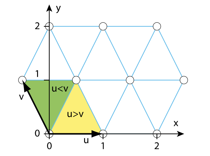
1. Given a point $p=(x,y)$, transform it to a skewed coordinate system $(u,v)$.
   • The vectors $u,x$ are parallel, but $v$ is rotated 30 degrees counter-clockwise from $y$.
   • We also scale the grid in the $y$ direction so that the points fall on integer positions in $y$.
2. For $(u,v)$, we can find the following:
   • The lower left vertex of the cell is at $(u_0,v_0)=(\text{floor}(u),\text{floor}(v))$.
   • Local coordinates of the point are $(u_f,v_f)=(u-u_0,v-v_0)$
   • Check if $u_f>v_f$, to see if the point is in the right or left triangle of the skewed grid box.
     • If $u_f>v_f$, we’re in the right side, so the three corners are
       $$(u_0,v_0),(u_0,v0+1),(u_0+1,v_0+1)$$
     • If $u_f<v_f$, we’re in the left side, so the three corners are
       $$(u_0,v_0),(u_0+1,v_0),(u_0+1,v_0+1)$$

We can transform the points in the $(u,v)$ coordinate system to the $(x,y)$ coordinate system once the corner points are found.

The transformation is as follows:

$$\{\begin{array}{l}u=x+y/2\\ v=y\end{array}\{\begin{array}{l}x=u-v/2\\ y=v\end{array}$$

This slightly stretches the grid a bit, but doesn’t produce any visual artifacts.

Under this stretched grid, we can use 0.8 instead of 0.75 for the radial decay.

Sample code can be found below.

Simplex Noise: Sample Code

// Gradient Generation
// Generate gradient vecors using a permutation polynomial
float permute(float x, float b) {
    float h = mod(x, 289.0f);
    return mod((34.0 * h + b) * h, 289.0);
}
vec2 gradient(vec2 p) {
    float B1 = 7.f;
    float B2 = 6.f;
    
    float x = permute(permute(p.x, B1) + p.y, B1) / 288.f;
    float y = permute(permute(p.x, B2) + p.y, B2) / 288.f;
    
    // Our permutation function gives us a value in [0,1].
    // Convert this to a gradient vector that can go in any direction. 
    return normalize(vec2(x,y) - vec2(0.5, 0.5));
}
 
// Perlin Noise:
vec2 xy_to_uv(vec2 xy) {
    return vec2(xy.x + xy.y * 0.5, xy.y);
}
vec2 uv_to_xy(vec2 uv) {
    return vec2(uv.x - uv.y * 0.5, uv.y);
}
 
float noise(vec2 p) {
    vec2 uv = xy_to_uv(p);
    
    // Find the corners of my simplex
    vec2 uv0 = floor(uv);
    vec2 luv = fract(uv); // Local
    vec2 uv1 = uv0;
    uv1 += vec2(step(luv.y, luv.x), step(luv.x, luv.y));
    vec2 uv2 = uv0 + vec2(1., 1.);
    
    // Sample my gradient function
    vec2 g0 = gradient(uv0);
    vec2 g1 = gradient(uv1);
    vec2 g2 = gradient(uv2);
    
    // Compute my noise contributions
    vec2 v0 = p - uv_to_xy(uv0);
    float w0 = max(0.75 - dot(v0, v0), 0.);
    w0 = w0 * w0;
    w0 = w0 * w0;
    vec2 v1 = p - uv_to_xy(uv1);
    float w1 = max(0.75 - dot(v1, v1), 0.);
    w1 = w1 * w1;
    w1 = w1 * w1;
    vec2 v2 = p - uv_to_xy(uv2);
    float w2 = max(0.75 - dot(v2, v2), 0.);
    w2 = w2 * w2;
    w2 = w2 * w2;
    
    float n0 = w0 * dot(g0, v0);
    float n1 = w1 * dot(g1, v1);
    float n2 = w2 * dot(g2, v2);
 
    float n = n0 + n1 + n2;
    
    // Scale to [0,1]
    return (10.9 * n + 1.) / 2.;
}

Simplex Noise Image

Generating Noise (3D) §

The 3D case is similar to the 2D case, but instead of triangles, we’re now considering tetrahedrons.

1. Transform the point to skewed space
2. Find the cell we are in, which has 8 possible corners
3. Find the 4 closest corners in the cell, giving us our simplex
4. Generate a gradient for each corner
5. Transform all 4 corners back to unskewed space
6. Compute the radial falloff and gradient contribution
7. Compute and sum the noise values from all 4 corners
8. Scale the output to the desired range of values

Now, in our 3D case, we have the following transformation:

$$\{\begin{array}{l}u=y+z\\ v=x+z\\ w=x+y\end{array}\{\begin{array}{l}x=(-u+v+w)/2\\ y=(u-v+w)/2\\ z=(u+v-w)/2\end{array}$$

Then, for $(u,v,w)$, to find the 4 corners of our simplex, we compute

$$\begin{gathered} (u_0,v_0,w_0)=(\text{floor}(u),\text{floor}(v),\text{floor}(w)) \\ (u_3,v_3,w_3)=(u_0+1,v_0+1,w_0+1) \end{gathered}$$

And can find the other two corners by computing

$$(u_f,v_f,w_f)=(u-u_0,v-v_0,w-w_0)$$

The other two corners are found by adding 1 to the coordinate with the largest coordinate value, and adding 1 to the coordinates with the 2 largest coordinate values. This can be done with step functions!

Then, we can compute for each corner $i\in \{0,1,2,3\}$,

• $r^2=v_i\cdot v_i$, where $v_i$ is the vector from the corner to our point
• $w=\max (0.5-r^2,0)$
• $n_i=w^3(g_i\cdot v_i)$
• $\text{Noise}=n_0+n_1+n_2+n_3$

To generate gradients in 3D, we can use a Fibonacci Sphere, which defines a mapping from an integer $k$ to one of $N$ uniformly spaced vectors on a sphere.

$$\begin{array}{r}k\in \{0,1,N-1\}\\ \theta =4\pi k/(1+\sqrt{5})\\ z=\cos \varphi =1-2(k+1/2)/N\\ w=\sin \varphi =\sqrt{1-z^2}\\ x=w\cos \theta \\ y=w\sin \theta \end{array}$$

Derivatives of Simplex Noise §

One of the major advantages of simplex noise is that it’s structure lets us analytically compute its derivative. This can be useful for a variety of effects, and is made possible as we are summing the noise contributions, instead of intepolerating them (like in Perlin Noise).

For 2D noise, we can find the derivatives by summing

$$n_i=w^4(g_i\cdot v_i)⟹\nabla n_i=w^4\cdot g_i-8w^3(g_i\cdot v_i)v_i$$

And for 3D noise, we can find the derivative by summing

$$n_i=w^3(g_i\cdot v_i)⟹\nabla n_i=w^3{g}_i-6w^2(g_i\cdot v_i)v_i$$

Noise Techniques §

Multifractal Combinations §

To get noise that is more detailed, we can consider overlaying noise on top of itself at different scales. Noise scaled up can define larger features, and noise scaled down can define smaller details.

The most generic way this can be done is as follows:

$$F(p)=\sum _{i=0}^k{2}^{-i}\text{noise}(2^i\bar{p})$$

Make sure to divide by 2 after if you want to normalize back to [0,1].

To get more interesting results, it may help to weigh later terms on a value dependent on previous terms, instead of a fixed value only dependent on $i$.

$$F(p)=\sum _{i=0}^k{A}_i\text{noise}(2^{i}p)A_i=A(i,F_{k_1})$$

One example of this is setting $A_k=F_{k-1}$, which gives good results for terrain.

Warping §

Another technique we can perform with noise is warping. Here, we push the noise input coordinate around, to create a “warping” effect on the resultant image.

One way we could do this is by displacing each term of the noise sum with the summed gradients of the previous terms.

float k = 3.;
float c = 0.;
vec2 disp = vec2(0);
 
for (float i = 0.; i < k; i++) {
    // We displace what we're sampling from the noise function here
    vec2 trans_xy = pow(2., i) * (xy + disp);
    c += pow(2., -i) * noise(trans_xy);
    // Update our displacement based on the sampled gradient
    disp += dnoise(trans_xy);
}
    
c /= 2.;

A sample using what we’ve made from this section! https://www.shadertoy.com/view/tfdXRB

Scatterings §

A scattering is a random distribution of positions. They occur naturally and frequently in the real world:

• The distribution of trees on a landspace
• The appearance of gravel
• The distribution of rain drops on a window

Here, we explore how we can generate scatterings in a procedural shader.

Groundwork §

Given a 2D plane, what we want is a seemingly random distribution of points where no two points are closer than $d$ distance of each other. This distance $d$ is variable, and lets us configure the appearance of our distribution.

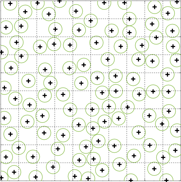
To do this, we can split our area into cells, and for each cell, compute a jitter that determines the location of a point. This jitter can be computed pseudorandomly using one of the previously mentioned hashing methods.

By smartly toggling the size of the jitter, we can get a distribution that looks similar to what we want!

But where do we compute these points? On the GPU, we can’t simply generate every point on every invocation of the pixel shader! This is simply too computationally expensive.

Of course, we could precompute the point set on the CPU, but we want to find an alternative using procedural shaders (as that’s the point of this book).

What we can do instead, is only generate points in regions close to any given pixel. This limits the number of points we need to generate, and only gives us points that are of interest (reasonably close to the pixel).

1. For a pixel, determine what grid cell we’re in
2. Iterate through nearby grid cells, and compute their jittered points
3. Perform a brute force search on these points to find which are the nearest.
   • Our jitter and search area must be compatible, such that there can’t possibly be closer points from cells outside of our search area.

Some research has found that using staggered grid cells, or forms of cells other than square may produce better results.

One example program using this technique is given below. It finds the closest point and computes the color as $1-2\ast d^2$, where $d$ is the distance to that point.

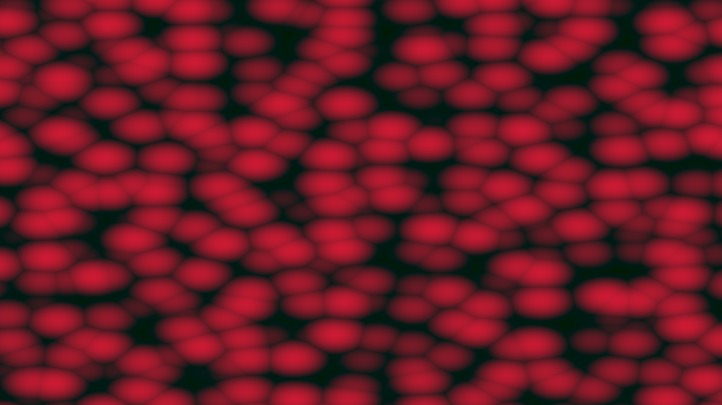
Example: Sample Code

// Gradient Generation
// Generate gradient vecors using a permutation polynomial
float permute(float x, float b) {
    float h = mod(x, 289.0f);
    return mod((34.0 * h + b) * h, 289.0);
}
vec3 gradient(vec3 p) {
    float B1 = 11.f;
    float B2 = 134.f;
    float B3 = 53.f;
    
    float x = permute(permute(permute(p.x, B1) + p.y, B1) + p.z, B1) / 288.f;
    float y = permute(permute(permute(p.x, B2) + p.y, B2) + p.z, B2) / 288.f;
    float z = permute(permute(permute(p.x, B3) + p.y, B3) + p.z, B3) / 288.f;
    
    // Our permutation function gives us a value in [0,1].
    // Convert this to a gradient vector that can go in any direction. 
    return normalize(vec3(x,y,z) - vec3(0.5, 0.5, 0.5));
}
 
void mainImage( out vec4 fragColor, in vec2 fragCoord )
{
    vec2 uv = fragCoord/iResolution.xy;
    vec3 xyz = vec3(uv * 15., iTime);
    
    // Config
    float jitter = 0.5f;
    
    // Determine the cell we are in
    vec3 cur_cell = floor(xyz);
    float c = 0.;
    
    float d1 = 100.;
    
    // Iterate through the neighbors of the cell
    for (int i = -1; i <= 1; i++) {
        for (int j = -1; j <= 1; j++) {
            for (int k = -1; k <= 1; k++) {
                vec3 cell = cur_cell + vec3(i,j,k);
 
                // Compute the pseudorandom point from that cell
                vec3 jitter_vec = gradient(cell) * jitter;
                vec3 point = cell + vec3(0.5) + jitter_vec;
 
                // Compute distance to this point
                float d = length(point - xyz);
 
                // Update d1, d2. D1 is distance to closest, D2
                // is 2nd closest
                d1 = (d < d1) ? d : d1;
            }
        }
    }
    
    c = 1. - 2. * d1 * d1;
    
    
    // Output to screen
    vec3 color = mix(vec3(0.1), vec3(0.8, 0.1, 0.2), c);
    fragColor = vec4(color, 1.);
}