Interpolation

Motivation

Consider a function $f(x)$ defined along the interval $[a,b]$. While we may be able to calculate it by hand, in practice, computers are unable to calculate all possible types of functions - and in these cases, it’s necessary to approximate the function $f(x)$.

A common way to do this is by approximating $f(x)$ using a polynomial

$$P_n(x)=a_0+a_{1}x+a_2{x}^2+a_3{x}_3+\cdots +a_n{x}^n$$

As the existence of these polynomials is guaranteed, granted we have continuity (see below).

Theorem: Weierstrass Approximation

If $f$ is a function that is continuous on the interval $[a,b]$, then for any $ϵ>0$, there exists a polynomial $P(x)$ such that for all $x\in [a,b]$,

$$|f(x)-P(x)|<ϵ$$

In other words, there exists a polynomial that can become infitesminally close to our function $f(x)$.

One of the most popular polynomial approximations out there is the Taylor Series approximation.

Supposing that $f$ is differentiable $n$ times, then its Taylor Series approximation about $x_0$ is given as

$$f(x)\approx P_n(x)=f(x_0)+f^{\prime }(x_0)(x-x_0)+\cdots +f^n(x_0)\frac{(x-x_0{)}^n}{n!}$$

This approximation is good, but is typically only used for error estimation, as it has a few issues.

• This approximation requires $f$ to be differentiable $n$-times, limiting the functions we can approximate.
• This approximation is only good for approximations around $x_0$!

Below, we explore alternative, more practical ways to approximate $f$.

The Interpolation Problem

The Interpolation Property

One way we can approximate functions is by using interpolation.

Given $(n+1)$ distinct nodes $\{x_i{\}}_{i=0}^n$ along the function’s domain, interpolation aims to find a polynomial $P_n(x)$ such that for all $0\le i\le n$,

$$P_n(x_i)=f(x_i)$$

In other words, the polynomial guarantees equality at all points $x_i$, and approximates the function elsewhere. Such a function is said to satisfy the interpolation property.

This polynomial must have the minimum degree needed to achieve this. This gives us some notion of uniqueness for interpolating polynomials - otherwise, without this restriction, we could construct infinitely many polynomials that interpolate $f$.

We typically want to minimize our degree, so we can minimize error with our approximation.

Example: Non-Uniqueness of Interpolators

Let $P_n(x)$ have the interpolating property. Then, we can create a polynomial of higher degree with the same interpolating property.

$$Q_n(x)=P_n(x)+\prod _{i=0}^n(x-x_i{)}^{v_i}{v}_i\ge 1$$

This argument could be repeatedly applied to obtain higher and higher degrees!

The following theorem sets an upper bound on the degree needed for such a polynomial.

Theorem: Interpolation - Maximum Degree Needed

If $\{x_i{\}}_{i=0}^n$ are $(n+1)$ distinct nodes, then for any set of $(n+1)$ values $f(x_0),f(x_1),\dots f(x_n)$, there exists a unique polynomial $P_n(x)$ with degree $\le n$ such that the interpolation property holds.

How can we explicitly construct such polynomials?

Lagrange Interpolating Polynomials

One way we can explicitly construct such polynomials is by using the Lagrange Interpolating Polynomial.

Suppose we have $\{x_i{\}}_{i=0}^n$ distinct nodes. Then, for any $0\le j\le n$, define the polynomial

$$l_j(x)=\frac{(x-x_0)(x-x_1)\dots (x-x_{j-1})(x-x_{j+1})\dots (x-x_n)}{(x_j-x_0)(x_j-x_1)\dots (x_j-x_{j-1})(x_j-x_{j+1})\dots (x_j-x_n)}$$

Note how we don’t include the $(x-x_j)$ and $(x_j-x_j)$ terms.

By this definition, we know that given any $l_j$ polynomial, called the basis polynomials, for any $0\le i\le n$,

$$l_j(x)=\{\begin{array}{ll}0& i\ne j\\ 1& i=j\end{array}$$

And furthermore, the degree of each $l_j$ polynomial is $n$.

Summing the $l_j$ polynomials, we can obtain the Lagrange Polynomial.

$$P_n(x)=\sum _{j=0}^{n}f(x_j)l_j(x)$$

Which, by property of the basis functions, is guaranteed to be equal to $f(x_j)$ at $x=x_j$ (all other basis functions will drop to 0 except the $l_j$ function).

Example: Lagrange Interpolating Polynomials

Let $x_0=2,x_1=3,x_2=5$, and let $f=1/n$. We find

$$f(x_0)=\frac{1}{2}f(x_1)=\frac{1}{3}f(x_2)=\frac{1}{5}$$

We first determine each $l_j$ polynomial.

$$\begin{array}{rl}& l_0(x)=\frac{(x-3)(x-5)}{(2-3)(3-5)}=\frac{1}{3}(x^2-8x+15)\\ & l_1(x)=\frac{(x-2)(x-5)}{(3-2)(3-5)}=-\frac{1}{2}(x^2-7x+10)\\ & l_2(x)=\frac{(x-2)(x-3)}{(5-2)(5-3)}=\frac{1}{6}(x^2-5x+6)\end{array}$$

We use these to create our Lagrange Polynomial.

$$\begin{array}{rl}{P}_3(x)& =\frac{1}{6}(x^2-8x+15)-\frac{1}{6}(x^2-7x+10)+\frac{1}{30}(x^2-5x+6)\\ & =\frac{1}{30}(x^2-10x+31)\end{array}$$

Lagrange Form Benefits

The Lagrange Form can particularly be useful if we have the same fixed points $\{x_i{\}}_{i=0}^{n+1}$ for different $f$‘s, as our basis functions remain the same! This will avoid computational costs

Compare this with Newton’s Form (later), where we’d have to recalculate all the divided differences.

Newton’s Form of Interpolation

Another way we can explicitly construct such polynomials is by using Newton’s Form of Interpolation.

This method attempts to find the polynomial in the form

$$P_n(x)=a_0+a_1(x-x_0)+x_2(x-x_0)(x-x_1)+\cdots +a_n\prod _{j=0}^{n-1}(x-x_j)$$

Where $a_0\dots a_n$ are constants we are attempting to find.

Suppose we have $\{x_i{\}}_{i=0}^n$ distinct nodes. Then, we define the $k^{th}$ divided difference of $f$.

• The zeroth divided difference of $f$ at $x_i$ is $$f[x_i]=f(x_i)$$
• The first divided difference of $f$ at $x_i,x_{i+1}$ uses the zeroth divided difference. $$f[x_i,x_{i+1}]=\frac{f[x_{i+1}]-f[x_i]}{x_{i+1}-x_i}=\frac{f(x_{i+1})-f(x_i)}{x_{i+1}-x_i}$$
• The second divided difference of $f$ at $x_i,x_{i+1},x_{i+2}$ uses the first divided difference. $$f[x_i,x_{i+1},x_{i+2}]=\frac{f[x_{i+1},x_{i+2}]-f[x_i,x_{i+1}]}{x_{i+2}-x_i}$$
• The $k^{th}$ divided difference of $f$ at $x_i,x_{i+1},\dots x_{i+k}$ uses the $(k-1{)}^{th}$ divided difference. $$f[x_i,x_{i+1},\dots x_{i+k}]=\frac{f[x_{i+1},x_{i+2},\dots x_{i+k}]-f[x_i,x_{i+1},\dots x_{i+k-1}]}{x_{i+k}-x_i}$$

The below diagram illustrates how we would calculate the $4^{th}$ divided difference on $x_0,x_1,x_2,x_3$.

graph LR
0[x<sub>0</sub>];
1[x<sub>1</sub>];
2[x<sub>2</sub>];
3[x<sub>3</sub>];

0 -.-> 4["f[x<sub>0</sub>]"];
1 -.-> 5["f[x<sub>1</sub>]"];
2 -.-> 6["f[x<sub>2</sub>]"];
3 -.-> 7["f[x<sub>3</sub>]"];

4 & 5 -.-> 8["f[x<sub>0</sub>,x<sub>1</sub>]"];
5 & 6 -.-> 9["f[x<sub>1</sub>,x<sub>2</sub>]"];
6 & 7 -.-> 10["f[x<sub>2</sub>,x<sub>3</sub>]"];

8 & 9 -.-> 11["f[x<sub>0</sub>,x<sub>1</sub>,x<sub>2</sub>]"];
9 & 10 -.-> 12["f[x<sub>1</sub>,x<sub>2</sub>,x<sub>3</sub>]"];

11 & 12 -.-> 13["f[x<sub>0</sub>,x<sub>1</sub>,x<sub>2</sub>,x<sub>3</sub>]"];

These divided differences become our coefficients! Using $x=x_k$, we can find our coefficient as

$$a_k=f[x_0,x_1,\dots x_k]$$

Giving us polynomial

$$P_n(x)=f[x_0]+\sum _{k=1}^n\left(f[x_0,\dots x_k]\cdot \prod _{j=0}^{k-1}(x-x_j)\right)$$

Note that by our above uniqueness theorem, the polynomial obtained here should be the same as the Lagrange Polynomial.

Theorem: Divided Differences and Permutations

If $y_0,y_2,\dots y_k$ is any permutation of our points $x_0,x_1,\dots x_k$, then their divided differences are the same.

$$f[y_0,y_1,\dots y_k]=f[x_0,x_1,\dots x_k]$$

Example: Newton's Interpolation

Let $x_0=2,x_1=3,x_2=5$, and let $f=1/n$. We find

$$f(x_0)=\frac{1}{2}f(x_1)=\frac{1}{3}f(x_2)=\frac{1}{5}$$

We find our divided differences.

$$\begin{array}{rl}& f[x_0]=f(x_0)=1/2\\ & f[x_1]=f(x_1)=1/3\\ & f[x_2]=f(x_2)=1/5\\ & f[x_0,x_1]=\frac{1/3-1/2}{3-2}=-1/6\\ & f[x_1,x_2]=\frac{1/5-1/3}{5-3}=-1/15\\ & f[x_0,x_1,x_2]=\frac{-1/15-(-1/6)}{5-2}=1/30\end{array}$$

We now use these differences to find our polynomial.

$$\begin{array}{rl}{P}_3(x)& =f[x_0]+f[x_0,x_1](x-x_0)+f[x_0,x_1,x_2](x-x_0)(x-x_1)\\ & =\frac{1}{2}-\frac{1}{6}(x-2)+\frac{1}{30}(x-2)(x-3)\end{array}$$

This is equivalent to the polynomial we found using Lagrange’s Method!

Newton Form Benefits

The Newton Form can particularly be useful if we need to add more fixed points for the same $f$. This will keep our divided differences the same, as we can use these already calculated divided differences to easily calculate the extra differences we need!

Compare this with Lagrange, where we’d have to recalculate all the basis functions if we add a new node.

Errors in Interpolation

Let $f$ have $n+1$ continuous derivatives on some interval $[a,b]$.

Let $P_n(x)$ be the interpolating polynomial at $(n+1)$ distinct nodes $\{x_i{\}}_{i=0}^n$. Then, for all $x\in [a,b]$, there exists an error $\delta (x)$ such that

$$f(x)-P_n(x)=f^{n+1}(\delta (x))\frac{{\prod }_{j=0}^n(x-x_j)}{(n+1)!}$$

We prove this fact below.

Proof

Let $x\in [a,b]$.

Suppose $x$ is one of the interpolating nodes. Then, we are done.

Suppose $x$ is not one of the interpolating nodes. Define

$$w(y)=\prod _{j=0}^n(y-x_j)$$

Which has degree $n+1$, with leading term $1\cdot y^{n+1}$.

We use this to define the function with $n+1$ continuous derivatives

$$F(y)=f(y)+P_n(y)-\lambda w(y)$$

Where $\lambda$ is chosen such that $F(x)=0$.

$$\lambda =\frac{f(x)-P_n(x)}{w(x)}$$

We know that because $x$ is not an interpolating node, $\lambda$ is defined.

Because of this, we know that $F(x)=0$, and $F(x_i)=0$ as well as all terms drop to 0! So, $F$ drops to 0 at $x,x_0,x_1,\dots x_n$.

Without loss of generalization, assume $x,x_0,x_1,\dots x_n$ are ordered. Then, by Rolle’s theorem, there must exist points between each consecutive pair such that $F^{\prime }(x)=0$ - in other words, there are $(n+1)$ distinct nodes where $F^{\prime }$ will drop to 0.

• Reapplying Rolle’s theorem, there must be $n$ distinct nodes where $F^{\prime \prime }$ will drop to 0.
• Reapplying Rolle’s theorem, there must be $(n-1)$ distinct nodes with $F^{\prime \prime \prime }$ will drop to 0.
• …

Continuing this way, we find that $F^{n+1}=0$ at some point, which we’ll call $\delta (x)$.

$$\begin{array}{rl}{F}^{n+1}(\delta (x))& =f^{n+1}(\delta (x))-P_n^{n+1}(\delta (x))-\lambda w^{n+1}(x)\\ & =f^{n+1}(\delta (x))-0-\lambda (n+1)!\\ & =f^{n+1}(\delta (x))-\frac{f(n)-P_n(x)}{w(x)}(n+1)!\end{array}$$

This can be refactored to obtain the above result.

Hermite Interpolation

Problem Stated

Above, we saw that given $(n+1)$ distinct nodes, we can form a polynomial that equals our function $f$ at these points! Now, what if we had more information about $f$ at these nodes, like $f$‘s derivatives? Could we create a polynomial that interpolates $f$ on these derivatives as well?

Consider the following example.

Example: Finer Interpolations of $f$

Find a $P(x)$ such that

$$\begin{array}{r}P(0)=f(0)=-1\\ P(1)=f(1)=0\\ P^{\prime }(1)=f^{\prime }(1)=-1\end{array}$$

Notice how we now have 2 conditions at the same node!

It’s definitely possible to find an interpolating polynomial! Plugging our values into the polynomial $P(x)=a_0+a_{1}x+a_2{x}^2$, we get a system of equations! Solving for it, we can find the polynomial

$$P(x)=-1+3x-2x^2$$

Note how in the above example, it seems reasonable to expect that as we have 3 conditions, the degree of our polynomial is $\le 2$. But this is not necessarily the case! Consider the following:

$$\begin{array}{r}{P}^{\prime }(0)=f^{\prime }(0)=c\\ P^{\prime }(1)=f^{\prime }(1)=d\end{array}$$

With 2 conditions, we may expect to find a polynomial with degree $\le 1$. But such a polynomial isn’t possible when $c\ne d$ (we’ll need a higher degree)! Moreover, even if $c=d$, we do not have enough information to produce a unique polynomial!

So, it’s definitely possible to interpolate values of $f(x)$ and $f^{\prime }(x)$ simultaneously, but additional conditions are needed to ensure the existence of a unique $P(x)$.

This problem is known as hermite interpolation, and is formally stated as follows. Consider the $l+1$ distinct nodes $x_0,\dots x_l$ with the strict ordering $x_0<x_1<x_2\cdots <x_l$.

We want to find a polynomial $P_n(x)$, whose degree is $\le n$ such that

$$P_n^i(x_j)=f^i(x_j)0\le i\le m_j-1,0\le j\le l$$

Such a polynomial is known as a hermite polynomial.

Where every node has $m_j$ conditions (derivatives). In other words, we need a polynomial which will equal all of the given derivatives for nodes $x_0\dots x_l$ provided!

Note that this means for a given problem, we have $m_0+m_1+\cdots +m_l$ conditions. As the number of unknowns in $P_n(n)=n+1$, we need $n+1$ to be equal to this sum! So, if we have the following number of unknown values (or less), we can guarantee uniqueness!

$$n=m_0+m_1+\cdots +m_l-1$$

Generalized Newton’s Form of Interpolation

Let’s reconsider our above example from another perspective.

Observation: Generalizing Newton's Form

Define non-distinct nodes (note how they’re now non-distinct) $x_0=0$, $x_1=1$, $x_2=1$. Let’s attempt to use Newton’s form of interpolation to find

$$\begin{array}{rl}{P}_2(x)& =f[x_0]+f[x_0,x_1](x-x_0)+f[x_0,x_1,x_2](x-x_0)(x-x_1)\\ & =f(0)+\frac{f(1)-f(0)}{1-0}(x-0)+f[0,1,1](x-0)(x-1)\\ & =-1+x+f[0,1,1]x(x-1)\end{array}$$

We can use Newton’s method to get this far normally, but we don’t know what to do with a divided difference on repeated elements! However, we’ve seen from our earlier example that we can find our polynomial as

$$P(x)=-1+3x-2x^2=-1+x-2x(x-1)$$

So we should expect $f[0,1,1]=-2$. Expanding our divided difference, we normally should expect

$$f[0,1,1]=\frac{f[1,1]-f[0,1]}{1-0}=f[1,1]-1$$

So $f[1,1]=-1$! Interestingly enough, this is precisely equal to $f^{\prime }(1)$! This suggests that there is a connection between our divided difference with repeated elements, and $f$‘s derivative at these repeated values!

In fact, given a divided difference

$$f[x,\tilde{x}]=\frac{f[\tilde{x}]-f[x]}{\tilde{x}-x}$$

If we take the limit as $\tilde{x}\to x$, we’ll get our derivative!

$$\underset{\tilde{x}\to x}{\lim }f[x,\tilde{x}]=f^{\prime }(x)$$

Thus, it makes sense that $f[x,x]=f^{\prime }(x)$! While we won’t formally prove it, we’ll state this observation in the following lemma.

Lemma: Generalizing Newton's Form

Let $x_0,x_1,x_2,\dots x_n$ be non-distinct nodes with the ordering $x_0\le x_1\le x_2\le \cdots \le x_n$. Then for a function continuous on $n$ derivatives $f\in C^n$, the $n^{th}$ order divided difference satisfies

$$f[x_0,x_1,\dots x_n]=\{\begin{array}{ll}\frac{f[x_1,x_2,\dots x_n]-f[x_0,x_1,\dots x_{n-1}]}{x_n-x_0}& x_0\ne x_n\\ \frac{f^n(x_0)}{n!}& x_0=x_n\end{array}$$

Note that if $x_0=x_n$, then all the nodes are the same due to the ordering of the nodes that we force.

This lemma lets us find divided differences on non-distinct nodes! Suppose we have conditions on the same node $x_i$ for $x_0,x_1,\dots x_l$. Define node $z_j$ to represent any single condition on some node $x_i$.

$$\{z_0,z_1,z_2,z_3,z_4,\dots \}=\{x_0,x_0,\dots ,x_1,\dots ,\}$$

Note that this number is equal to $n+1$, or $m_0+m_1+\cdots +m_l$.

Then, using Newton’s Form, our required polynomial is given as

$$P_n=f[z_0]+f[z_0,z_1](x-z_0)+f[z_0,z_1,\dots ,z_n]\prod _{i=0}^{n-1}(x-z_i)$$

Where we can use the above lemma to solve for the divided differences.

Consider the following example.

Example: Newton's Form for Hermite Interpolation

Find the Hermite polynomial using

$$f(0)=1f^{\prime }(0)=2f(2)=-1f^{\prime }(2)=3$$

First, note that there are two distinct nodes, 0 and 2. We’ll denote them as

$$x_0=0x_1=2$$

Furthermore, note that both nodes have 2 conditions, $m_0=2$, $m_1=2$.

We have all information up to our highest derivative for each node,so we can guarantee uniqueness of our polynomial!

We define our total notes, including repetitions, and use this to find our polynomial.

$$\{z_0,z_1,z_2,z_3\}=\{x_0,x_0,x_1,x_1\}$$

We find the divided differences as

$$\begin{array}{rl}& f[z_0]=f[x_0]=1\\ & f[z_1]=f[x_0]=1\\ & f[z_2]=f[x_1]=-1\\ & f[z_3]=f[x_1]=-1\\ & f[z_0,z_1]=f[x_0,x_0]=\frac{f^{\prime }(x_0)}{1!}=2\\ & f[z_1,z_2]=f[x_0,x_1]=\frac{f(x_1)-f(x_0)}{x_1-x_0}=\frac{-1-1}{2-0}=-1\\ & f[z_2,z_3]=f[x_1,x_1]=\frac{f^{\prime }(x_1)}{1!}=3\\ & f[z_0,z_1,z_2]=f[x_0,x_0,x_1]=\frac{f[x_0,x_1]-f[x_0,x_0]}{x_1-x_0}=\frac{-1-2}{2-0}=-\frac{3}{2}\\ & f[z_1,z_2,z_3]=f[x_0,x_1,x_1]=\frac{f[x_0,x_1]-f[x_1,x_1]}{x_1-x_0}=\frac{3+1}{2}=2\\ & f[z_1,z_2,z_3,z_4]=f[x_0,x_0,x_1,x_1]=\frac{f[x_0,x_1,x_1]-f[x_0,x_0,x_1]}{x_1-x_0}=\frac{2+3/2}{2}=\frac{7}{4}\end{array}$$

We put these together to findour polynomial! We know our polynomial is given as

$$\begin{array}{rl}{P}_3(x)& =f[z_0]+f[z_0,z_1](x-z_0)+f[z_0,z_1,z_2](x-z_0)(x-z_1)+f[z_0,z_1,z_2](x-z_0)(x-z_1)(x-z_2)\\ & =1+2x-\frac{3}{2}{x}^2+\frac{7}{4}{x}^2(x-2)\end{array}$$

Example: Newton's Form for Hermite Interpolation (2)

Suppose we find the hermite polynomial $P(x)$ such that $P^i(x_0)=f^i(x_0)$ for all $0\le i\le n$. Note that in this case, we only have one distinct node.

Because all of our $z_i$ terms are equal to the same $x_0$, when we write out our polynomial, we get

$$P_n(x)=f(x_0)+\frac{f^{\prime }(x_0)}{1!}(x-x_0)+\cdots +\frac{f^n(x_0)}{n!}(x-x_0{)}^n$$

This is, interestingly enough, the truncated Taylor series expansion of $f$ at $x_0$!

Theorem: Error Estimate on Hermite Polynomials

Consider $f\in C^{N+1}([a,b])$, the function continuous on $n$ derivatives along the interval $[a,b]$. Furthermore, consider polynomial with degree $\le N+1$ such that for $(l+1)$ distinct nodes $x_0,\dots x_l\in [a,b]$,

$$P_N^i(x_j)=f^i(x_j)\forall 0\le i\le m_{j-1},0\le j\le l$$

A polynomial approximating the nodes at the conditions given

and $m_0+m_1+\dots m_l=N+1$, then $\forall x\in [a,b]$, there exists an $\delta (x)\in (a,b)$ such that

$$f(x)-P_N(x)=\frac{f^{N+1}({\delta }_N(x))}{(N+1)!}\prod _{j=0}^l(x-x_j{)}^{m_j}$$

This estimates our error on hermite polynomials!

Issues with Interpolation

Below, we discuss issues that we face when interpolating polynomials.

Runge’s Phenomena

When interpolating a function with high degree polynomials, interpolations on equally spaced points can create oscillations along the edges of the interval being interpolated. This is known as Runge’s Phenomena.

Consider the following function, commonly known as the Runge Function

$$f(x)=\frac{1}{1+25x^2}$$

Now, consider the interpolating polynomial on $(n+1)$ equally-spaced nodes, with degree $\le n$. We have the following polynomials.

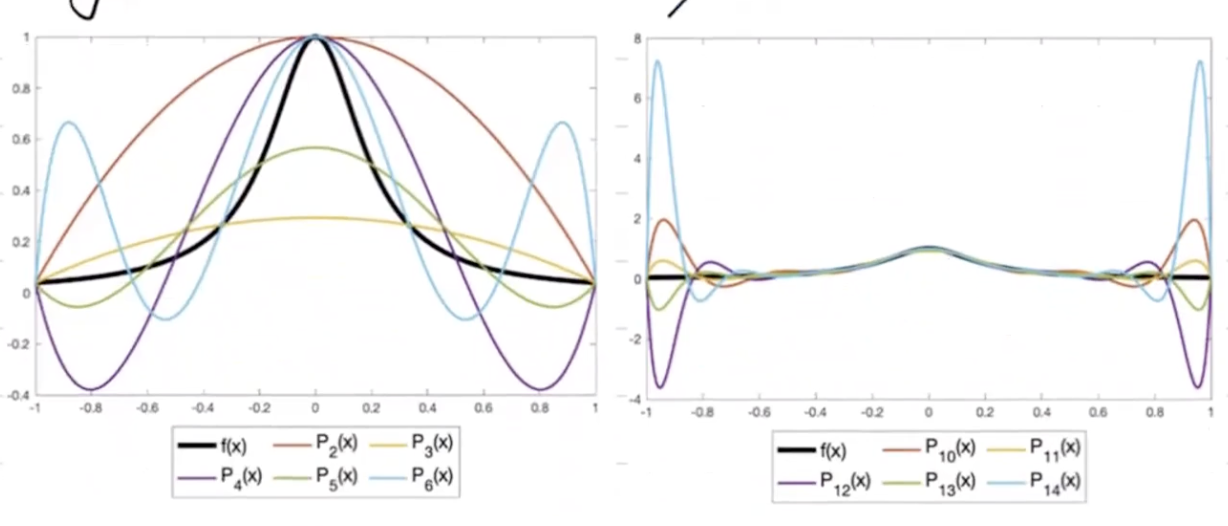
We can see that as we increase the degree of our polynomial, we get larger and larger oscillations at the end of the interval! This creates a ton of error.

How could we resolve this issue?

Resolving Runge’s Phenomena: Chebyshev Nodes

One way to resolve this issue is to pick non-equidistant nodes that will prevent oscillations from occurring around the edges! By concentrating our nodes around the edges, we make constrain the polynomial more so that it cannot oscillate.

In fact, one example of how we could choose these nodes is Chebyshev nodes, which are distributed more densely near the edges of the interval than the interior.

Resolving Runge’s Phenomena: Splines

Another way we could resolve this issue is by using piecewise interpolating polynomials! By combining polynomials together that interpolate different portions of our interval, we can minimize the maximum degree polynomial we use.

This is the idea behind splines! A spline of degree $k$ having $n+1$ knots $t_0,t_1,\dots t_n$ is a function $s(x)$ with the following properties:

1. On each interval between knots $[t_{i-1},t_i)$, $s(x)$ is a polynomial of degree $\le k$.
2. $s(x)$ is continuous on $k-1$ derivatives in the interval $[t_0,t_n]$.

We call $t_i$‘s knots, as they serve as “connections” for our piecewise polynomials.

Example: Splines

Consider a spline of degree 1! Then, for all pairs of nodes, we’ll have piecewise lines approximating our function!

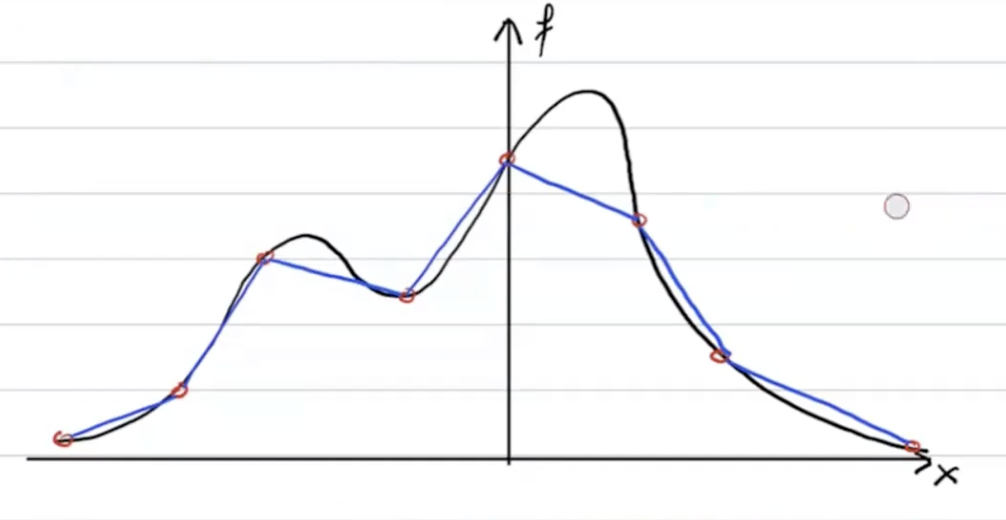
We don’t have to chooose our knots to be our interpolating nodes, though, this is quite a convenient choice.

One of the most commonly used types of splines is the cubic spline ($k=3$)! In such a spline, each piecewise polynomial $s_i(x)$ on $x\in [t_i,t_{i+1})$ has degree $\le 3$.

Furthermore, to be interpolating, the following must hold:

1. All polynomials in a spline must satisfy

   $$\begin{array}{r}{s}_i(t_i)=y_i\forall 0\le i\le n-1\\ s_{n-1}(t_n)=y_n\end{array}$$

   In other words, they must equal our nodes at their given value, and furthermore, our last polynomial should also match our last node as well.

2. Our spline must be continuous up to 2 derivatives, meaning

   $$\begin{array}{r}{s}_{i-1}(t_i)=s_i(t_i)=y_i\forall 1\le i\le n-1\\ s_{i-1}^{\prime }(t_i)=s_i^{\prime }(t_i)=y_i\forall 1\le i\le n-1\\ s_{i-1}^{\prime \prime }(t_i)=s_i^{\prime \prime }(t_i)=y_i\forall 1\le i\le n-1\end{array}$$

   In other words, our polynomials’ derivatives (up to the 2nd) must match with the polynomials they’re connected to.

As we have $n$ degree 3 polynomials, we have $4n$ unknowns! However, summing up the information needed for the interpolation above, we only have $4n-2$ conditions (equations), which is not enough information!

One common way to address this is by setting boundary conditions for the polynomials.

• Natural (Free) Boundaries: Setting the 2nd derivatives at the boundaries to be 0 - $s^{\prime \prime }(t_0)=s^{\prime \prime }(t_n)=0$.
• Clamped Boundaries: Setting $s^{\prime }(t_0)=f^{\prime }(t_0)$ and $s^{\prime }(t_n)=f^{\prime }(t_n)$.

Using natural boundaries, we will have to solve the system $Az=b$, where $z=[z_1,z_2,\dots z_{n-1}{]}^T\in {\mathbb{R}}^{n-1}$ and

$$A=\left[\begin{array}{ccccc}\frac{h_0+h_1}{3}& \frac{h_1}{6}& 0& 0& \dots \\ \frac{h_1}{6}& \frac{h_1+h_2}{3}& \frac{h_2}{6}& 0& \dots \\ 0& \frac{h_2}{6}& \ddots & \ddots & \\ 0& 0& \ddots & & \end{array}\right]b=\left[\begin{array}{c}\frac{y_2-y_1}{h_1}-\frac{y_1-y_0}{h_0}\\ \frac{y_3-y_2}{h_2}-\frac{y_2-y_1}{h-1}\\ ⋮\\ \frac{y_n-y_{n-1}}{h_{n-1}}-\frac{y_{n-1}-y_{n-2}}{h_{n-2}}\end{array}\right]$$

With our splines being given in the equation

$$s_i(x)=z_{i+1}\frac{(x-t_i{)}^3}{6h_i}+z_i\frac{(t_{i+1}-x{)}^3}{6h_i}+\left(\frac{y_{i+1}}{h_i}-\frac{z_{i+1}{h}_i}{6}\right)(x-t_i)+\left(\frac{y_i}{h_i}-\frac{z_i{h}_i}{6}\right)(t_{i+1}-x)$$

Where $h_i=t_{i+1}-t_i$ for all $0\le i\le n-1$, and $z_0=z_n=0$.

In MATLAB, we can solve this system using the spline function!