Differential Systems

In this section, we combine differential equations and linear algebra to produce differential systems.

Linear Differential Systems

Introduction

An $n$-dimensional differential system is defined as

$$\frac{d\vec{x}}{dt}=\vec{f}(t,\vec{x})$$

where

$$\frac{d\vec{x}}{dt}=\left[\begin{array}{c}{x}_1^{\prime }(t)\\ x_2^{\prime }(t)\\ ⋮\\ x_n^{\prime }(t)\end{array}\right]\vec{f}=\left[\begin{array}{c}{f}_1\\ f_2\\ ⋮\\ f_n\end{array}\right]$$

In other words, we have $n$ unknown functions in terms of $n$ given functions. We want to find a solutions to

$$\vec{x}=(x_1,x_2,\dots ,x_n)$$

We can often convert higher order differential equations into differential systems, which may be easier to solve!

For simplicity, we will only be working with first order linear systems.
Let $x_1,x_2,\dots ,x_n$ be our unknown function. A first order linear system is given as

$$\begin{array}{rl}& \frac{d{x}_1}{dt}=a_{11}(t)x_1+a_{12}(t)x_2+\cdots +a_{1n}(t)x_n+f_1(t)\\ & \frac{d{x}_2}{dt}=a_{21}(t)x_1+a_{22}(t)x_2+\cdots +a_{2n}(t)x_n+f_2(t)\\ & ⋮\\ & \frac{d{x}_n}{dt}=a_{n1}(t)x_1+a_{n2}(t)x_2+\cdots +a_{nn}(t)x_n+f_n(t)\end{array}$$

where $a_{ij},f_k$ are functions on $t$. Note that in these systems, all unknown functions are given in terms of their first derivative.

We represent differential systems in matrix form, as so:

$$A=\left[\begin{array}{ccc}{a}_{11}(t)& \dots & a_{1n}(t)\\ a_{21}(t)& \dots & a_{2n}(t)\\ ⋮& & ⋮\\ a_{nn}(t)& \dots & a_{nn}(t)\end{array}\right]\vec{x}=\left[\begin{array}{c}{x}_1\\ x_2\\ ⋮\\ x_n\end{array}\right]\vec{f}=\left[\begin{array}{c}{f}_1\\ f_2\\ ⋮\\ f_n\end{array}\right]$$ $$\frac{d\vec{x}}{dt}=A(t)\vec{x}+\vec{f}$$

Solutions to Differential Systems

To solve a differential system is to find a vector $\Phi (t)$ such that its entries (which are functions on $t$) satisfy our differential system

$$\frac{d\vec{x}}{dt}=A(t)\vec{x}+\vec{f}(t)$$

Oftentimes, we want to find a fundamental matrix to our differential system, which is a matrix of solutions $\{{\Phi }_1,{\Phi }_2,\dots ,{\Phi }_h\}$ such that

$$\left[\begin{array}{cccc}{\Phi }_1& {\Phi }_2& \dots & {\Phi }_h\\ \downarrow & \downarrow & \dots & \downarrow \end{array}\right]$$

such that each column is a solution, and the linear combination of all column vectors represents all possible solutions to our linear system.

Note: Given a fundamental matrix, we can actually find the system corresponding to this matrix of solutions!

Example: System from Fundamental Matrix

Suppose ${\Phi }_1,{\Phi }_2$ are solutions to a homogeneous differential system. What is the differential system?

We know that because our functions ${\Phi }_1,{\Phi }_2$ are solutions, they satisfy

$$\frac{d{\Phi }_1}{dt}=A(t){\Phi }_1\frac{d{\Phi }_2}{dt}=A(t){\Phi }_2$$ $$\to \left[\begin{array}{cc}\frac{d{\Phi }_1}{dt}& \frac{d{\Phi }_1}{dt}\\ \downarrow & \downarrow \end{array}\right]=A(t)\left[\begin{array}{cc}{\Phi }_1& {\Phi }_2\\ \downarrow & \downarrow \end{array}\right]$$

Thus, we can easily solve for $A(t)$ by performing matrix operations!

$$A(t)=\left[\begin{array}{cc}\frac{d{\Phi }_1}{dt}& \frac{d{\Phi }_1}{dt}\\ \downarrow & \downarrow \end{array}\right]{\left[\begin{array}{cc}{\Phi }_1& {\Phi }_2\\ \downarrow & \downarrow \end{array}\right]}^{-1}$$

Example: Finding the General Solution

Suppose we have differential system

$$\frac{d\vec{x}}{dt}=A(t)\vec{x}+\vec{f}(t)$$

Defined on interval $I=(a,b)$.

Now say we have solutions to differential system

$$u(t)=\left[\begin{array}{c}t+e^t\\ 1\end{array}\right]v(t)=\left[\begin{array}{c}1+e^t\\ 1\end{array}\right]w(t)=\left[\begin{array}{c}{e}^t\\ t\end{array}\right]$$

Find the general solution of this differential system.

Note that we cannot simply add our solutions together, as the system may not be homogeneous.

However, we see that subtracting our solutions will give us solutions to the homogeneous differential system!

$$u-vv-ww-u$$

Thus, if we use this to find the general solution for the homogeneous system, and then add a particular solution, we will find out general solution!

Thus, let’s choose

$${\Phi }_1=u-v{\Phi }_2=v-w$$

as our homogeneous general solution. We see their Wronskian is $W=-(t-1{)}^2$, so they only form a FSoS on $t\ne 1$.

Assuming that $t\ne 1$, therefore, we find our general solution to be

$$\vec{x}=c_1{\Phi }_1+c_2{\Phi }_2+w$$

Theorem: Solutions to Homogeneous Systems

Let $\frac{d\vec{x}}{dt}=A(t)\vec{x}+\vec{f}(t)$ be an $n$-dimensional differential system, such that $\vec{f}(t)=0$.

Then, the set of all solutions to the homogeneous system forms an $n$-dimensional vector space. We can thus choose $n$ functions $\{{\Phi }_1(t),{\Phi }_2(t),\dots ,{\Phi }_n(t)\}$ that span this vector space.

Note that because FSoS span the same solution space, there must necessarily exist a change of basis matrix that maps one to the other.

We know that such a matrix is a fundamental matrix if its determinant, otherwise known as its Wronskian, is not 0 on the entire interval on which the differential system is defined.

This is very similar to Fundamental Set of Solutions!

Luckily, we don’t have to check the Wronskian for all $t_0\in I$, by the following theorem:

Theorem: The Wronskian

If the Wronskian of $n$ solutions is 0 for some $t_0\in I$, then the Wronskian of these $n$ solutions is 0 for all $t_0\in I$.

Similar to differential equations, we also have Natural Fundamental Set of Solutions (NFSoS) $\{N_1,N_2,\dots \}$ such that only the $i^{th}$ entry of $N_i$ is 1, all others 0.

Given a differential system with initial values, known as an initial value problem, how can we obtain a NFSoS?
Given a fundamental matrix $X(t)$, we can easily find NFSoS for value $t_0$ by taking

$$X(t)\cdot X^{-1}(t_0)$$

Furthermore, we can multiply our NFSoS by initial value problem ${\vec{x}}_0$ to easily find our solution.

This should intuitively make sense! At $t=t_0$, we obtain

$$X(t_0)\cdot X^{-1}(t_0)=I$$

Additionally, we see the following theorem for initial value problems.

Theorem: Existence and Uniqueness

Let $\frac{d\vec{x}}{dt}=A(t)\vec{x}+\vec{f}(t)$ be an $n$-dimensional differential system.

If all entries of $A(t)$ and $\vec{f}(t)$ are defined and continuous over some interval $I=(a,b)$, then given initial value problem

$$t_0\in I\overrightarrow{x_0}\in {\mathbb{R}}^n$$

Then there exists one and only one solution $\vec{x}(t)$ to the system such that $\vec{x}(t_0)=\overrightarrow{x_0}$.

Example: Existence and Uniqueness - Disproving Solutions

Show that $\Phi (t)=(t^2+t,\sin (t))$ is not a solution to any homogeneous 2-dimensional linear differential system defined on $(-1,1)$.

Suppose $\Phi (t)$ satisfies

$$\frac{d\Phi }{dt}=A(t)\Phi (t)$$

The existence and uniqueness theorem guarantees that for all values in $(-1,1)$, there exists one and only one solution.

Pick initial condition $x(0)=(0,0)$. We can easily say there is solution $x(t)=(0,0)$.
However, if we take $\Phi (0)=(0,0)$, we also obtain $(0,0)$! As the existence and uniqueness theorem states there is only one solution for IVP, so $\Phi$ cannot be a solution!

Example: Existence and Uniqueness - Properties of Solutions

Take differential system

$$\frac{d\vec{x}}{dt}=\left[\begin{array}{cc}\sin (t)& 0\\ 0& t^3\end{array}\right]\vec{x}(t)+\left[\begin{array}{c}\sin (t)\\ \sin (t)\end{array}\right]$$

Prove there is a solution $\vec{x}(t)$ defined on $\mathbb{R}$ which is an even function.

Suppose we have an initial value problem with solution $\vec{a}(t)$. Because $\vec{a}(t)$ is a solution, it satisfies

$$\frac{d\vec{a}}{dt}=\left[\begin{array}{cc}\sin (t)& 0\\ 0& t^3\end{array}\right]\vec{a}(t)+\left[\begin{array}{c}\sin (t)\\ \sin (t)\end{array}\right]$$

Now, define $\vec{z}(t)=\vec{a}(-t)$. Plugging this into the differential equation, we obtain

$$-\frac{d\vec{v}}{dt}=\left[\begin{array}{cc}\sin (t)& 0\\ 0& t^3\end{array}\right]\vec{v}(-t)+\left[\begin{array}{c}\sin (t)\\ \sin (t)\end{array}\right]$$

Now, using the fact that $\sin (t)$ and $t^3$ are odd functions, we substitute

$$\sin (t)=-\sin (-t)t^3=-(-t{)}^3$$ $$-\frac{d\vec{v}}{dt}=\left[\begin{array}{cc}-\sin (-t)& 0\\ 0& -(-t{)}^3\end{array}\right]\vec{v}(-t)+\left[\begin{array}{c}-\sin (-t)\\ -\sin (-t)\end{array}\right]$$

Applying a change of variables $s=-t$, we see that

$$\frac{d\vec{v}}{dt}=\left[\begin{array}{cc}\sin (s)& 0\\ 0& s^3\end{array}\right]\vec{v}(s)+\left[\begin{array}{c}\sin (s)\\ \sin (s)\end{array}\right]$$

We see that $\vec{v}(t)$ is a solution! However, as the Existence and Uniqueness Theorem guarantees a unique solution for this initial value problem,

$$\vec{v}(t)=\vec{a}(t)\to \vec{a}(-t)=\vec{a}(t)$$

Thus, $\vec{a}(t)$ is an even function!

Differential Equations as Systems

Given any arbitrary differential equation, we can represent it as a differential system. This is important, as all linear differential equations will translate to first order systems, which may considerably simplify solving!

To represent an equation $L[y]=f$ as a system, choose $x_i$ to be our functions, where each $x_i$ corresponds to some derivative of $y$ under the order of the equation. Then, find what $x_i^{\prime }$ is to create your matrix.

What we are essentially doing is creating an isomorphism between the equation and system! So, if we find a solution to our equation, we can transform it into a solution for our system!

Some examples are given below.

Example: Equations as Systems (1)

Take second order differential equation

$$y^{\prime \prime }+y=e^t$$

We know from constant differential equations that we have FSoS to homogeneous differential equation $\{\sin (t),\cos (t)\}$, and finding particular solution $y_p=\frac{e^t}{2}$, we have general solution

$$y(t)=c_1\sin (t)+c_2\cos (t)+\frac{e^t}{2}$$

Let’s now relate this to differential systems.
Define $x_1=y$, $x_2=y^{\prime }$ to obtain differential system

$$\begin{array}{rl}& \frac{d{x}_1}{dt}=y^{\prime }=x_2\\ & \frac{d{x}_2}{dt}=y^{\prime \prime }=-y+e^t=-x_1+e^t\\ & \to \frac{d\vec{x}}{dt}=\left[\begin{array}{cc}0& 1\\ -1& 0\end{array}\right]\vec{x}+\left[\begin{array}{c}0\\ e^t\end{array}\right]\end{array}$$

Note that the characteristic polynomial of $A$ is the same as the characteristic polynomial of the differential equation $p(z)$!

Given our previously found solution, we know we have solution

$$\vec{x}=c_1\left[\begin{array}{c}\sin (t)\\ \cos (t)\end{array}\right]+c_2\left[\begin{array}{c}\cos (t)\\ \sin (t)\end{array}\right]+e^t\left[\begin{array}{c}1\\ 1\end{array}\right]$$

Example: Equations as Systems (2)

$$t^2{y}^{\prime \prime }-2y=t^3$$

Convert the following differential equation to a system.

Let $x_1=y,x_2=y^{\prime }$. We find that

$$\begin{array}{rl}& x_1^{\prime }=y^{\prime }=x_2\\ & x_2^{\prime }=y^{\prime \prime }=\frac{1}{t^2}(2y+t^3)=\frac{2}{t^2}{x}_1+t\end{array}$$

And use this to find matrices $A(t)$ and $\vec{f}(t)$ for our system

$$A(t)=\left[\begin{array}{cc}0& 1\\ \frac{2}{t^2}& 0\end{array}\right]\vec{f}(t)=\left[\begin{array}{c}0\\ t\end{array}\right]$$

Example: Equations as Systems (3)

$$t{y}^4-t^2{y}^{\prime \prime }+\cos (t)y^{\prime }=e^{2t}$$

Convert the following differential equation to a system.

Define $x_1=y,x_2=y^{\prime },x_3=y^{\prime \prime },x_4=y^{\prime \prime \prime }$. We find that

$$\begin{array}{rl}& x_1^{\prime }=y^{\prime }=x_2\\ & x_2^{\prime }=y^{\prime \prime }=x_3\\ & x_3^{\prime }=y^{\prime \prime \prime }=x_4\\ & x_4^{\prime }=y^{\prime \prime \prime \prime }=\frac{e^{2t}}{t}+t{y}^{\prime \prime }-\frac{\cos (t)}{t}{y}^{\prime }=\frac{e^{2t}}{t}+t{x}_3-\frac{\cos (t)}{t}{x}_2\end{array}$$

And use this to find matrices $A(t)$ and $\vec{f}(t)$ for our system

$$A(t)=\left[\begin{array}{cccc}0& 1& 0& 0\\ 0& 0& 1& 0\\ 0& 0& 0& 1\\ 0& -\frac{\cos (t)}{t}& t& 0\end{array}\right]\vec{f}(t)=\left[\begin{array}{c}0\\ 0\\ 0\\ \frac{e^{2t}}{t}\end{array}\right]$$

Constant Linear Systems

Suppose we have differential system

$$\frac{d\vec{x}}{dt}=A(t)\vec{x}+\vec{f}(t)$$

such that $A(t)$ is a constant matrix (a matrix whose entries are all constants). We’ll define these systems as constant differential systems.

Note that there are more constant systems than there are constant differential equations. Our previous method of finding the solution for a constant equation may not work for all systems.

How do we solve these equations?

Solutions to Homogeneous Systems

Take homogeneous constant system

$$\frac{d\vec{x}}{dt}=A(t)\vec{x}$$

Now, observe that if we take the exponential of matrix $A$, defined as

$$e^A=\sum _{n=0}^{\infty }\frac{A^n}{n!}$$

Taking the exponential of $At$ offers really convenient solutions to our system!

We can prove this by computing its derivative.

$$\begin{array}{rl}& \frac{d}{dt}{e}^{At}\\ & =\frac{d}{dt}\left(I+At+A^2\frac{t^2}{2!}+A^3\frac{t^3}{3!}\dots \right)\\ & =A+A^{2}t+A^3\frac{t^2}{2!}+A^4\frac{t^3}{3!}\dots \\ & =A{e}^{At}\end{array}$$

Furthermore, we see that the determinant of the exponential matrix is never 0, as

$$det(e^{At})=e^{tr(A)t}\ne 0$$

So, the columns of $e^{At}$ always forms a FSoS for our constant differential system! We can thus find our FSoS by finding the Jordan Form of $A$ and taking the matrix exponential, to obtain $e^{At}$!

Theorem: Solutions to Constant Homogeneous Systems

The FSoS constant homogeneous differential system

$$\frac{d\vec{x}}{dt}=A\cdot \vec{x}$$

can always be found by finding the column vectors of the matrix exponential $e^{At}$.

Working in reverse, how can we find $e^{At}$?

1. Because all fundamental matrices can be transformed to one another via a constant matrix, we know that for some fundamental matrix $\Phi (t)$, $$e^{At}=\Phi (t)\cdot B$$ Furthermore, we know that at $t=0$, $e^0=I$! $$e^0=\Phi (0)\cdot B\to B={\Phi }^{-1}(0)$$ So, we know our fundamental matrix $\Phi (t)=e^{At}$ if $\Phi (0)=I$, and if it is not the exponential, we can easily find $e^{At}$ by solving for $B$!

   Thus, we may sometimes be able to use our experience with constant differential equations to easily find our exponential matrix!

2. Alternatively, we now that if we have the NFSoS about $t=0$, $$e^{At}=N_{0}I+N_{1}A$$ We can prove this. We know that by definition, at $t_0$ where the NFSoS is based, $$N_0(t_0)=1N_0^{\prime }(t_0)=0N_1(t_0)=0N_1^{\prime }(t_0)=1$$ Additionally, any derivative of $e^{At}$ yields $\frac{d^i}{d{t}^i}{e}^{At}=A^i{e}^{At}$.
   Thus, at $t=0$, $$e^0=I=(1)I+(0)A$$ $$\frac{d}{dt}{e}^{At}=A{e}^{At}\to A{e}^0=A=(0)I+(1)A$$ We can generalize this with the following theorem.

Theorem: Finding the Matrix Exponential

Suppose we have constant homogeneous differential system

$$\frac{d\vec{x}}{dt}=A\cdot \vec{x}$$

And let $L[y]$ be the $n^{th}$ order differential equation with characteristic polynomial equal to the characteristic polynomial of $A$.

If $N_0,N_1,\dots ,N_{n-1}$ is a NFSoS for $L[y]$ at $t=0$, then

$$e^{At}=N_{0}I+N_{1}A+N_2{A}^2+\cdots +N_{n-1}{A}^{n-1}$$

All we need to know about matrix $A$ is its characteristic polynomial to find the system’s solution! Note that $N_0,N_1,\dots$ are polynomials and not matrices.

Note: We can find the NFSoS easily by taking the Wronskian of a FSoS $W$, and multiply it with $W^{-1}(0)$!

Proof

Consider the derivative operator $D=\frac{d}{dt}$. We know that

$$D(e^{At})=A{e}^{At}{D}^2(e^{At})=A^2{e}^{At}$$

Take the linear operator $L=q(D)$ of the differential equation. We know that

$$L[e^{At}]=p(A)e^{At}$$

Furthermore, as $p(A)$ is the characteristic polynomial of $A$, it is 0 by the Cayley-Hamilton theorem.

$$L[e^{At}]=0$$

Thus, all entries of $e^{At}$ are solutions to $L[y]=0$!

Take NFSoS $N_0,N_1,\dots ,N_{n-1}$. We know that we can form the columns of $e^{At}$ as a linear combination of these solutions. This forms linear combination

$$e^{At}=B_{0}I+B_1{N}_1+\cdots +B_{n-1}{N}_{n-1}$$

Where $B_i$ are matrices we want to find. We can solve each $B_i$, as at $t=0$,

$$D^i(e^{At})=A^i{e}^{At}\to A^i{e}^0=A^i=B_i=B_i{N}_i^i(0)$$

Example: Solutions to Homogeneous Systems (1)

Let there be differential system

$$\frac{d\vec{x}}{dt}=A(t)\vec{x}+\vec{f}(t)A=\left[\begin{array}{cc}2& 0\\ 0& 3\end{array}\right]$$

We can easily find the FSoS for this system by finding $e^{At}$!

$$e^{At}=\left[\begin{array}{cc}{\sum }_{n=0}^{\infty }\frac{(2t{)}^n}{n!}& 0\\ 0& {\sum }_{n=0}^{\infty }\frac{(3t{)}^n}{n!}\end{array}\right]=\left[\begin{array}{cc}{e}^{2t}& 0\\ 0& e^{3t}\end{array}\right]$$

Thus, we find FSoS

$$\left[\begin{array}{c}{e}^{2t}\\ 0\end{array}\right]\left[\begin{array}{c}0\\ e^{3t}\end{array}\right]$$

Note: We should expect this, as this system is equivalent to the differential equations

$$x_1^{\prime }=2x_1{x}_2^{\prime }=3x_2$$

Whose solutions can very easily be seen as

$$x_1=e^{2t}{x}_2=e^{3t}$$

Example: Solutions to Homogeneous Systems (2)

Let’s take a more complicated example. Let there be differential system

$$\frac{d\vec{x}}{dt}=A(t)\vec{x}+\vec{f}(t)A=\left[\begin{array}{cc}3& 1\\ 0& 4\end{array}\right]$$

Find a FSoS for this system.

We begin by finding the Jordan form of $A$. We take the characteristic polynomial of $A$

$$p(z)=det(A-zI)=(3-z)(4-z)$$

To find eigenvalues 3 and 4. We then find an eigenvector for each eigenvalue:

$$\begin{array}{rl}& \lambda =3(A-3I)v=0\to v=(c,0)c\in \mathbb{R}\\ & \lambda =4(A-4I)=0\to v=(c,c)c\in \mathbb{R}\end{array}$$

Choose $c=1$. We have diagonalized $A$ as

$$A=\left[\begin{array}{cc}1& 1\\ 0& 1\end{array}\right]\left[\begin{array}{cc}3& 0\\ 0& 4\end{array}\right]{\left[\begin{array}{cc}1& 1\\ 0& 1\end{array}\right]}^{-1}$$

Now, we take the exponential of $At$ to find our FSoS.

$$e^{At}=\left[\begin{array}{cc}1& 1\\ 0& 1\end{array}\right]\left[\begin{array}{cc}{e}^{3t}& 0\\ 0& e^{4t}\end{array}\right]\left[\begin{array}{cc}1& -1\\ 0& 1\end{array}\right]=\left[\begin{array}{cc}{e}^{3t}& e^{4t}-e^{3t}\\ 0& e^{4t}\end{array}\right]$$

Solutions to Non-Homogeneous Systems

Just like with differential equations, to find a general solution to a non-homogeneous system, we find the general solution to the corresponding homogeneous system, and add that to a specific solution of the non-homogeneous system.

How do we find this specific solution?

Variation of Parameters

Recall the variation of parameters technique, where given general solution to homogeneous equation $\{y_1,y_2,\dots ,y_n\}$, we find specific solution

$$y_P=u_1{y}_1+u_2{y}_2+\dots u_n{y}_n$$

where $u_i$ are functions on $t$.

With differential systems, we perform variation of parameters similarly. Let us have differential system

$$\frac{d\vec{x}}{dt}=A\vec{x}+\vec{f}(t)$$

where $\Phi (t)$ is a fundamental matrix for the corresponding homogeneous system

$$\frac{d\vec{x}}{dt}=A\vec{x}$$

Suppose ${\vec{x}}_1,{\vec{x}}_2,\dots ,{\vec{x}}_n$ are the solution vectors of $\Phi (t)$. We want to find a specific solution such that

$${\vec{x}}_P=u_1{\vec{x}}_1+u_2{\vec{x}}_2+\cdots +u_n{\vec{x}}_n$$

Where $u_i$ are functions on $t$. We can rewrite this as

$${\vec{x}}_P=\Phi (t)\vec{u}(t)$$

Where

$$\vec{u}(t)=\left[\begin{array}{c}{u}_1\\ u_2\\ ⋮\\ u_n\end{array}\right]$$

Now, because ${\vec{x}}_P$ is a solution to the non-homogeneous solution, it must satisfy

$$\begin{array}{rl}& \frac{d{\vec{x}}_P}{dt}={\Phi }^{\prime }(t)\vec{u}(t)+\Phi (t){\vec{u}}^{\prime }(t)\\ & \frac{d{\vec{x}}_P}{dt}=A{\vec{x}}_P+\vec{f}(t)\end{array}$$

Because we know by assumption that $\Phi (t)$ is a solution to the homogeneous system, it must be true that ${\Phi }^{\prime }(t)=A\Phi (t)$. So, we obtain

$${\Phi }^{\prime }(t)\vec{u}(t)+\Phi (t){\vec{u}}^{\prime }(t)=A\Phi (t)\vec{u}(t)+\Phi (t){\vec{u}}^{\prime }(t)=A{\vec{x}}_P+\Phi (t){\vec{u}}^{\prime }(t)$$

Because this must be equal to

$$A{\vec{x}}_P+\Phi (t){\vec{u}}^{\prime }(t)=\frac{d{\vec{x}}_P}{dt}=A{\vec{x}}_P+\vec{f}(t)$$

This forces $\Phi (t){\vec{u}}^{\prime }(t)=\vec{f}(t)$! Furthermore, as $\Phi (t)$ is a fundamental matrix, it is invertible, so we can find

$${\vec{u}}^{\prime }(t)={\Phi }^{-1}(t)\vec{f}(t)\to \vec{u}(t)=\int {\Phi }^{-1}(t)\vec{f}(t)dt$$

Finally, we can find our specific solution as

$${\vec{x}}_P=\Phi (t)\cdot \int {\Phi }^{-1}(t)\vec{f}(t)dt$$

Theorem: Variation of Parameters

Suppose we have constant non-homogeneous solution

$$\frac{d\vec{x}}{dt}=A\vec{x}+\vec{f}(t)$$

and fundamental matrix to the corresponding homogeneous system $\Phi (t)$.

Then, there exists specific solution ${\vec{x}}_P$ such that

$${\vec{x}}_P=\Phi (t)\cdot \int {\Phi }^{-1}(t)\vec{f}(t)dt$$

Furthermore, if we have initial value problem $\vec{x}(t_0)={\vec{x}}_0$, we have specific solution

$${\vec{x}}_P={\vec{x}}_0+\Phi (t)\cdot {\int }_{t_0}^t{\Phi }^{-1}(t)\vec{f}(t)dt$$

Laplace Transforms

Recall from Ordinary Differential Equations, we defined the Laplace Transform as

$$F(s)=\mathcal{L}\{f\}={\int }_0^{\infty }{e}^{-st}f(t)dt$$

which is a one-to-one linear transformation mapping functions on $t$ to functions on $s$.

We can apply this similarly to differential systems, where

$$\mathcal{L}\{\vec{f}\}=\left[\begin{array}{c}\mathcal{L}\{f_1\}\\ \mathcal{L}\{f_2\}\\ ⋮\end{array}\right]$$

In other words, we apply the Laplace transform to each component of the vector.

Suppose we have differential system

$$\frac{d\vec{x}}{dt}=A\vec{x}+\vec{f}\vec{x}(0)=\vec{v}$$

To solve it using Laplace transforms, let $\mathcal{L}\{\vec{x}\}=\vec{X}(s)$ be the Laplace transform of $\vec{x}$, and $\mathcal{L}\{\vec{f}\}=\vec{F}(s)$ be the Laplace transform of $\vec{f}$.

Then,

$$\begin{array}{rl}& \mathcal{L}\left\{\frac{d\vec{x}}{dt}\right\}=\{A\vec{x}\}+\mathcal{L}\{\vec{f}\}\\ & \to s\vec{X}-\vec{v}=A\vec{X}+\vec{F}\\ & \to \vec{X}(sI-A)=\vec{F}+\vec{v}\\ & \to \vec{X}=(sI-A{)}^{-1}(\vec{F}+\vec{v})\end{array}$$

We can take the inverse, as for sufficiently large values of $s$, $det(sI-A)\ne 0$ (and we just need the Laplace transform to work for some interval $s$)!

Note that we can take the matrix $A$ out, as it is a constant matrix, so $A\vec{x}$ is really just taking a linear combination of $x_1,x_2,\dots ,x_n$.

Example 1: Laplace Transforms

$$\frac{d\vec{x}}{dt}=\left[\begin{array}{cc}0& 1\\ -6& 5\end{array}\right]\vec{x}+\left[\begin{array}{c}0\\ 2e^t\end{array}\right]\vec{x}(0)=\vec{v}=(1,1)$$

Let $\vec{X}$ be the Laplace transform of $\vec{x}$. Then, we find

$$\vec{F}(s)=\mathcal{L}\{\vec{f}\}=\left[\begin{array}{c}0\\ \frac{2}{s-1}\end{array}\right]sI-A=\left[\begin{array}{cc}s& 0\\ 0& s\end{array}\right]-\left[\begin{array}{cc}0& 1\\ -6& 5\end{array}\right]=\left[\begin{array}{cc}s& -1\\ 6& s-5\end{array}\right]$$ $$\vec{X}(s)=(sI-A{)}^{-1}(\vec{F}(s)+\vec{v})=\frac{1}{s^2-5s+6}\left[\begin{array}{cc}s-5& 1\\ -6& 5\end{array}\right]\left(\left[\begin{array}{c}0\\ \frac{2}{s-1}\end{array}\right]+\left[\begin{array}{c}1\\ 1\end{array}\right]\right)=\left[\begin{array}{c}\frac{1}{s-1}\\ \frac{1}{s-1}\end{array}\right]$$ $$\vec{x}(t)=\left[\begin{array}{c}{e}^t\\ e^t\end{array}\right]$$

We found a specific solution!

Non-Linear Differential Systems

Consider a non-linear differential system. As it is not linear, we cannot combine known solutions to form new solutions. In other words, our solution set does not span a vector space!

Because of this, we would have to explicitly find different solutions to solve the system, which is oftentimes not worth it!

So, instead of explicitly finding solutions, we instead describe the shape of solutions!

Given a non-linear differential system, we want to know what behavior solutions to the system take!

Autonomous Systems

Consider an autonomous system, which a differential system taking on the form

$$\frac{d\vec{x}}{dt}=\vec{f}(\vec{x})$$

where $\vec{x}=(x_1,x_2,\dots ,x_n)$ are functions on $t$, and $\vec{f}$ does not explicitly depend on $t$.

Note that autonomous systems can be both linear and non-linear! We first describe properties using linear systems (which we know), and generalize to non-linear systems.

For simplicity, we will only be working with non-linear autonomous systems. Given an autonomous system, we want to know the following:

1. Equilibrium solutions, and behaviors of solutions near the equilibrium solution.
2. Paths of solutions to the system, otherwise known as orbits.

Both of these are described below.

Equilibrium Solutions

Equilibrium and Stability

Given an autonomous system, a solution $\vec{\Phi }(t)$ to an autonomous system is stationary / equilibrium if it is a constant (unchanging) solution. In other words, if

$$\frac{d\vec{\Phi }}{dt}=0$$

Thus, to find an equilibrium solution, set the system’s derivatives to 0, and solve for the components of $\vec{x}$!

Example: Equilibrium Solutions (1)

$$\frac{dx}{dt}=(x-1)(y-1)\frac{dy}{dt}=(x+1)(y+1)$$

We find our stationary solutions by taking $x^{\prime }=y^{\prime }=0$.

$$(x-1)(y-1)=0(x+1)(y+1)=0$$

We perform a case analysis.

• Choosing $x=1$, we have $y=-1$.
• choosing $y=1$, we have $x=-1$.

Thus, our equilibrium solutions are

$$(1,-1)(-1,1)$$

Example: Equilibrium Solutions (2)

$$\frac{dx}{dt}=x{y}^2-x\frac{dy}{dt}=x\sin (\pi y)$$

We find our stationary solutions by taking $x^{\prime }=y^{\prime }=0$.

$$x(y^2-1)=0x\sin (\pi y)=0$$

We perform a case analysis.

• Choosing $x=0$, $y$ can be any value.
• Choosing $y=\pm 1$, $x$ can be any value.

Thus, we have stationary solutions

$$y=-1y=1x=0$$

where any point on the line is a stationary solution!

Furthermore, a stationary solution is semi-stationary if all but one of the coordinates are 0.

Now say we have a solution to differential system ${\vec{\Phi }}_0(t)$. We call ${\vec{\Phi }}_0$ a stable solution if (informally) any solution $\vec{\Phi }(t)$ that is sufficiently close to $\overrightarrow{{\Phi }_0}(t)$ for $t=0$ stays close to $\overrightarrow{{\Phi }_0}(t)$ for all $t$.

More formally, this is stated as $\forall ϵ>0$, there $\exists \delta >0$ such that

$$||\Phi (0)-{\Phi }_0(0)||<\delta \to ||\Phi (t)-{\Phi }_0(t)||<ϵ$$

for all $t$.

In other words, for all solutions in any ball (centered around our solution) of size $ϵ$, we can find a ball of size $\delta$ such that all functions starting within the $\delta$ ball stay within the $ϵ$ ball for all $t$!

In 2 dimensions, instead of a ball, we look at a disk (circle) around our solution.

Furthermore, a stable solution $\overrightarrow{{\Phi }_0}(t)$ is asymptotically stable, if any solution sufficiently close to $\overrightarrow{{\Phi }_0}(t)$ converges to $\overrightarrow{{\Phi }_0}(t)$.

Otherwise, our solution is unstable. Negating the earlier definition for stability, a solution is unstable if $\exists ϵ>0$, such that $\forall \delta >0$

$$||\Phi (0)-{\Phi }_0(0)||<\delta \nrightarrow ||\Phi (t)-{\Phi }_0(t)||<ϵ$$

We can find a $ϵ$ ball for which there is no $\delta$ ball!

Typically, with stable solutions, we are looking to see if solutions stay within a “tube” around our changing $\overrightarrow{{\Phi }_0}(t)$. However, for equilibrium solutions, we are just looking at a stationary disk / ball around $\overrightarrow{{\Phi }_0}(t)$!

Let’s now examine the stability of linear systems, and work to see how we can use that for non-linear systems!

Stability of Linear Equilibriums

Consider a linear system given by

$$\frac{d\vec{x}}{dt}=A\vec{x}$$

where $A$ is a constant matrix.

We can see that in these systems, the origin is always an equilibrium solution. Thus, with these systems, we are commonly interested in examining the stability of the equilibrium solution.

Example: Stable Equilibrium

$$A=\left[\begin{array}{cc}0& -3\\ 3& 0\end{array}\right]$$

Using our prior knowledge of constant linear systems, we know that our solution set to differential system comprises some combination of the functions $\{\sin (3t),\cos (3t)\}$.

Thus, all solutions will oscillate back in a periodic motion! So, while they will stay near the origin, they will never equal the origin, making the origin stable (but not asymptotically stable)!

Example: Asymptotically Stable Equilibrium

$$A=\left[\begin{array}{cc}-2& 0\\ 0& -3\end{array}\right]$$

Using our prior knowledge of constant linear systems, we can find the solution set of this differential system as

$$\left(e^{-2t},0\right)\left(0,e^{-3t}\right)$$

Now, say we have any arbitrary solution

$$\Phi (t)=c_1\left(e^{-2t},0\right)+c_2\left(0,e^{-3t}\right)$$

we see that as $t\to \infty$, $\Phi (t)\to 0$! What’s more, because the exponentials are negative, $\Phi (0)$ is the solution’s maximum value!

Thus, we see that our origin is stable, as all solutions near the origin stay near the origin (by converging inwards)!

More formally speaking, if we have an $ϵ$ ball, we know that all functions $\Phi (t)$ within this ball will never escape, as they are strictly decreasing! Thus, for all $ϵ$ balls, we choose a $\delta$ ball such that $\delta =ϵ$, as all functions within $\delta$ stay within $ϵ$.

Thus, we show that the origin is a stable equilibrium using $\delta /ϵ$! Furthermore, because all solutions converge to 0 as $t\to \infty$, the origin is asymptotically stable!

Using a similar idea, we observe that so long as our solution set consists only of negative exponentials, our solutions will always converge to the origin, giving us an asymptotically stable equilibrium!

Example: Unstable Equilibrium

$$A=\left[\begin{array}{cc}3& 0\\ 0& 2\end{array}\right]$$

Using our prior knowledge of constant linear systems, we can find the solution set of this differential system as

$$\left(e^{3t},0\right)\left(0,e^{2t}\right)$$

Now, say we have any arbitrary solution

$$\Phi (t)=c_1\left(e^{3t},0\right)+c_2\left(0,e^{2t}\right)$$

we see that for any solution such that $c_1$ and $c_2$ are not both 0, the solution diverges to $\infty$!

Thus, we see that the origin is unstable, as all solutions, no matter how close, diverge!

More formally speaking, we show that $\exists ϵ>0$, such that $\forall \delta >0$,

$$||\Phi (0)-{\Phi }_0(0)||<\delta \nrightarrow ||\Phi (0)-{\Phi }_0(0)||<ϵ$$

Say we pick a ball $ϵ=1$. Then, regardless of the $\delta$ ball we choose, we can pick a function within this ball

$$\left(\frac{\delta }{2}{e}^{3t},0\right)$$

such that as $t\to \infty$,

$$\underset{t\to \infty }{\lim }\left(\frac{\delta }{2}{e}^{3t},0\right)=(\infty ,0)>ϵ$$

In other words, we can always find a solution which will always drift away from the origin, no matter how close it starts to it!

Thus, our origin is an unstable solution.

There are lots of solutions which escape here! We just need to choose one to prove instability, however.

Using a similar idea, we observe that so long as we have any solution with a positive exponential, we will always have a set of solutions diverging to infinity, making our origin an unstable equilibrium!

Given the above examples, we can make the following observations:

1. When all of the solutions are combinations of negative exponentials, the origin is asymptotically stable.
2. When any singular solution is a positive exponential, the origin is unstable.

Thus, we see that the stability of our origin depends on which solution set comprises the system!

Thus, given that we can find solutions to linear systems using $A$‘s eigenvalues, it should be no surprise that $A$‘s eigenvalues can indicate the stability of the origin. We formalize this finding in the following theorem:

Theorem: Stability of Linear Systems

Suppose we have linear differential system

$$\frac{d\vec{x}}{dt}=A\vec{x}$$

where $A$ is a constant matrix.

Then, the system has equilibrium solution $\vec{0}$ (the origin), whose stability depends solely on the eigenvalues (denoted ${\lambda }_i$) of $A$, as so:

• If $Re({\lambda }_i)$ are all negative, then $\vec{0}$ is asymptotically stable.
• If $Re({\lambda }_i)$ are all non-positive, and the algebraic multiplicity of all $Re(\lambda )=0$ equals their geometric multiplicity, then $\vec{0}$ is stable (but not asymptotically stable).
• If $Re({\lambda }_i)$ is positive for any singular eigenvalue, then $\vec{0}$ is unstable.

Furthermore, all other solutions are stable if and only if $\vec{0}$ is stable.

One major application this comes up in is in determining precision of solutions!

Example: Margins of Error

Suppose we have a linear system

$$\frac{d\vec{x}}{dt}=A\vec{x}$$

We know that with initial conditions $\vec{x}(0)=(1,1)$, we can find a solution

$$e^{At}(1,1)$$

which describes how our initial values change over time.

However, in the real world, nothing is perfect! So, say we made a mistake in measuring our initial values, and have an error. Will our slightly-off solution remain a good estimate of our desired results?

We know if it will remain a good estimate if solutions in our system are stable, which we can determine based on $A$‘s eigenvalues.

Now, let $\vec{v}$ be our error. Because we have a linear system, we have solution

$$e^{At}((1,1)+\vec{v})$$

Thus, to find how our error changes over time, we can find

$$e^{At}\vec{v}$$

Note that if $A$ has all negative eigenvalues, our imprecise solution actually converges to our desired solution!

Stability of Non-Linear Equilibriums

Let’s now consider equilibrium for non-linear systems. How do we know if a given equilibrium is stable or unstable?

Let’s consider a one-dimensional case

$$\frac{d\vec{x}}{dt}=x(1-x)$$

We can easily find equilibrium points $x=0,1$. Tracing them on a number line, we can see how ${\vec{x}}^{\prime }$ behaves at different intervals along this line.

$$\{\begin{array}{ll}{\vec{x}}^{\prime }<0& (1,\infty )\\ {\vec{x}}^{\prime }>0& (0,1)\\ {\vec{x}}^{\prime }<0& (-\infty ,0)\end{array}-\infty \leftarrow 0\to 1\leftarrow \infty$$

From this, we can see that $x=1$ is a stable point (as points move towards it), whereas $x=0$ is an unstable point!
Note that we don’t actually care about the value of the derivative - we only care about the sign!

We now generalize this idea to higher-dimensions. Consider a non-linear differential system given by

$$\frac{d\vec{x}}{dt}=f(x,y)\frac{d\vec{y}}{dt}=g(x,y)$$

where $\vec{v}=(x,y)$.

Now consider some point in this system $\vec{P}$. We define

$$D_{ϵ}(\vec{P})=\{\vec{x}\in {\mathbb{R}}^n:||\vec{x}-\vec{P}||<ϵ\}$$

as the open ball (disk) around this point $\vec{P}$, the set of all points within a fixed distance of $\vec{P}$.

Now let $\vec{P}=(x_0,y_0)$ be an equilibrium point, and consider the values of the derivatives at a point very close to $\vec{P}$, which we’ll call $\vec{Q}$.

We can use tangent plane approximation to approximate the functions $f(x,y)$, $g(x,y)$ about $\vec{P}$ as

$$\begin{array}{rl}& f(x,y)\approx f(x_0,y_0)+f_x(x_0,y_0)(x-x_0)+f_y(x_0,y_0)(y-y_0)\\ & g(x,y)\approx g(x_0,y_0)+g_x(x_0,y_0)(x-x_0)+f_y(x_0,y_0)(y-y_0)\end{array}$$

Only for points close to $\vec{P}$!

Which allows us to approximate our system using the system:

$$\frac{d}{dt}\left(\genfrac{}{}{0ex}{}{x}{y}\right)=\left(\begin{array}{c}f(x_0,y_0)\\ g(x_0,y_0)\end{array}\right)+\left(\begin{array}{cc}{f}_x(x_0,y_0)& f_y(x_0,y_0)\\ g_x(x_0,y_0)& g_y(x_0,y_0)\end{array}\right)\left(\begin{array}{c}x-x_0\\ y-y_0\end{array}\right)$$

Using the fact that $\vec{P}$ is a stationary point, we know that functions $f$ and $g$ are 0 at $\vec{P}$. Furthermore, defining $\tilde{x}=\vec{x}-{\vec{x}}_0$, we see that

$$\frac{d\tilde{x}}{dt}=\frac{d\vec{x}}{dt}$$

Giving us system

$$\frac{d}{dt}\left(\genfrac{}{}{0ex}{}{\tilde{x}}{\tilde{y}}\right)=\left(\begin{array}{cc}{f}_x(x_0,y_0)& f_y(x_0,y_0)\\ g_x(x_0,y_0)& g_y(x_0,y_0)\end{array}\right)\left(\begin{array}{c}\tilde{x}\\ \tilde{y}\end{array}\right)$$

This is called the linearization of a non-linear system about a equilibrium point, where

$$J=\left(\begin{array}{cc}{f}_x(x_0,y_0)& f_y(x_0,y_0)\\ g_x(x_0,y_0)& g_y(x_0,y_0)\end{array}\right)$$

is called the Jacobian.

Using this linearization, we can see how points near our equilibrium point approximately behave! These behaviors are approximations, as our derivatives in the Jacobian are approximations of the actual derivatives.

Now that we’ve approximated a linear system, we can now use our earlier theorem with linear systems to determine the behavior of points around our equilibrium.

Theorem: Stability of Non-Linear Systems

Suppose we have a non-linear differential system

$$\frac{d\vec{x}}{dt}=\vec{f}(\vec{x})$$

With equilibrium points ${\vec{x}}_1,{\vec{x}}_2,\dots ,{\vec{x}}_n$.

Now say we have the linearized differential system about some equilibrium point ${\vec{x}}_i$.

$$\frac{d\vec{x}}{dt}=A\vec{x}$$

Then, we can determine the stability of the equilibrium point depending on the eigenvalues (denoted ${\lambda }_i$) of $A$, as so:

• If $Re({\lambda }_i)$ are all negative, then ${\vec{x}}_i$ is asymptotically stable.
• If $Re({\lambda }_i)$ is positive for any singular eigenvalue, then $\vec{0}$ is unstable.

Note that by the theorem, we cannot say anything when there is an eigenvalue of 0!

This is because as matrices with values close to one another have approximately the same eigenvalues, we can say positive eigenvalues stay positive and negative eigenvalues stay negative, but we cannot say anything about 0 eigenvalues!

Thus, we can say an equilibrium point is asymptotically stable or unstable, but cannot tell if it’s stable or not!

Example: Stability of Non-Linear Equilibrium

Define non-linear differential system

$$\frac{dx}{dt}=1-xy\frac{dy}{dt}=x-y^3$$

Solving for equilibrium points by letting

$$\frac{dx}{dt}=0\frac{dy}{dt}=0$$

We find the equilibrium points $(1,1),(-1,-1)$. We now determine their stability.

For $(1,1)$, we linearize the system by defining

$$\tilde{x}=x-1\tilde{y}=y-1$$

And calculating

$$\begin{array}{rl}& \frac{d\tilde{x}}{dt}=1-xy=1-(\tilde{x}+1)(\tilde{y}+1)=-\tilde{x}-\tilde{y}-\tilde{x}\tilde{y}\\ & \frac{d\tilde{y}}{dt}=(\tilde{x}+1)-(\tilde{y}+1{)}^3=\tilde{x}-({\tilde{y}}^3+3{\tilde{y}}^2+3\tilde{y})\end{array}$$

But we choose $\tilde{x}$ and $\tilde{y}$ so small that any power is extremely small! So, we’ll effectively ignore them (we’re approximating the functions) to obtain

$$\begin{array}{rl}& \frac{d\tilde{x}}{dt}=-\tilde{x}-\tilde{y}\\ & \frac{d\tilde{y}}{dt}=\tilde{x}-3\tilde{y}\end{array}$$

Note: We can just take the partial derivatives, but when doing that, this is in essence what we are doing!

Which is our linearized system! Taking matrix

$$A=\left[\begin{array}{cc}-1& -1\\ 1& -3\end{array}\right]$$

we calculate the eigenvalues as $-2,-2$, telling us that all solutions near the equilibrium converge to the equilibrium! So, $(1,1)$ is an asymptotically stable equilibrium.

For $(-1,-1)$, we perform a similar process, and linearize the system to obtain matrix

$$A=\left[\begin{array}{cc}1& 1\\ 1& -3\end{array}\right]$$

Giving us eigenvalues $-1\pm \sqrt{5}$. Because there is a positive eigenvalue, not all points will stay near the equilibrium, and the equilibrium is unstable.

Example: Stability of Non-Linear Equilibrium

Consider non-linear differential system

$$\frac{dx}{dt}=\sin (x+y)\frac{dy}{dt}=e^x-1$$

We find the equilibrium points

$$(0,n\pi ):n\in \mathbb{Z}$$

Additionally, we find the Jacobian by taking the partial derivatives of functions $f$ and $g$.

$$J=\left[\begin{array}{cc}\cos (x+y)& \cos (x+y)\\ e^x& 0\end{array}\right]$$

Now, we perform a case analysis to determine the stability of the points.

1. When $n$ is even, we obtain the Jacobian matrix

   $$\left[\begin{array}{cc}1& 1\\ 1& 0\end{array}\right]$$

   With eigenvalues $\frac{1\pm \sqrt{5}}{2}$, and as at least one is positive, these equilibrium points are unstable.

2. When $n$ is odd, we obtain the Jacobian matrix

   $$\left[\begin{array}{cc}-1& -1\\ 1& 0\end{array}\right]$$

   With eigenvalues $\frac{-1\pm \sqrt{3}i}{2}$, and as all eigenvalues have negative real parts, these equilibrium points are asymptotically stable.

Orbits and the Phase Plane

Orbits and Sinks/Sources

Take 2-dimensional autonomous system

$$\frac{dx}{dt}=f(x,y)\frac{dy}{dt}=g(x,y)$$

We will mainly work with 2-dimensional systems here, as higher dimensions are just too complicated!

We define the orbit of a solution $(x_0,y_0)$ as the path a solution takes over some time interval. Furthermore, we define an orbit as closed (periodic solution) when it equals itself on two separate time periods.

While both orbits and solutions describe the path, the solution tells us exact position at a time, whereas an orbit cannot!

We also use this definition of an orbit for further definitions of equilibrium points.
Given an equilibrium point, if orbits drift towards the point, it is a sink, and if orbits drift away from the point, it it is a source.

Otherwise, if an equilibrium is both a sink and source, it is a saddle.

Determining an orbit is fairly easy! Observe the following:

$$\frac{dy}{dt}\frac{1}{\frac{dx}{dt}}=\frac{g}{f}=\frac{dy}{dx}$$

Thus, we just need to solve $g/f$ to know find our slope at any point $(x_0,y_0)$, which can be traced to give us our orbit!
We may also be able to solve the resulting equation to obtain an ellipse curve, telling us the path shape taken by all orbits!

However, this method is not the only method to determine orbits!

Given any point $x_0,y_0$, we guarantee the existence of an orbit by the following theorem:

Existence and Uniqueness: Autonomous Systems (2-Dimensional)

Say we have autonomous system

$$\frac{dx}{dt}=f(x,y)\frac{dy}{dt}=g(x,y)$$

where $f,g$ are continuously differentiable on ${\mathbb{R}}^2$.

Then, for any point $P$ on ${\mathbb{R}}^2$, there exists one and only one solution $x(t),y(t)$ with $(x(0),y(0))=P$.

This theorem generalizes to $n$ dimensions!

Existence and Uniqueness: Autonomous Systems (n-Dimensional)

Say we have autonomous system given by

$$\frac{d\vec{x}}{dt}=\vec{f}(\vec{x})$$

Suppose that the partial derivatives of $\vec{f}$, given by $\frac{\partial f_i}{\partial x_j}$, are all continuous on some open set $U\subseteq {\mathbb{R}}^n$.

Then, for any $t_0\in \mathbb{R}$, and for any point $\vec{P}\in U$, there exists one and only one solution $\Phi (t)$ defined on some open interval $I$ containing $t_0$ such that

$$\Phi (t_0)=\vec{P}$$

This theorem also guarantees that periodic solutions obey closed curves. Otherwise, if we have periodic solution

$$\Phi (t+L)=\Phi (t)$$

which does not obey a closed curve, there would be multiple other solutions starting at the same point, which violates our theorem!

This can be formalized with the following theorem.

Theorem: Uniqueness of Orbits

Say we have autonomous system given by

$$\frac{d\vec{x}}{dt}=\vec{f}(\vec{x})$$

Suppose that the partial derivatives of $\vec{f}$, given by $\frac{\partial f_i}{\partial x_j}$, are all continuous on some open set $U\subseteq {\mathbb{R}}^n$.

Then, distinct orbits do not intersect - they cannot share the same points!
Furthermore, if the orbit of some solution $\Phi (t)$ a simple closed curve, equaling itself at some time $L$

$$\Phi (t)=\Phi (0)$$

and furthermore, does not contain an equilibrium point, then $\Phi (t)$ must be a periodic.

$$\Phi (L+t)=\Phi (t)$$

Proof (Intuition) $\vec{P}$.

Suppose we have two distinct orbits which sharing a point

Then, we can define these orbits such that at some time $t$, they’re both at that point, violating the existence and uniqueness theorem!

Orbits of Linear Systems

Just like before, we will first figure out how to determine the orbits for linear systems, and then generalize this to non-linear systems.

Consider a linear system given by

$$\frac{d\vec{x}}{dt}=A\vec{x}$$

where $A$ is a constant matrix.

Note that if we have an eigenvector $\vec{v}$ to matrix $A$, then we can find its solution as

$$e^{At}v=(I+At+\frac{A^2{t}^2}{2}+\dots )v=e^{\lambda t}v$$

and because $e^{\lambda t}$ is a scalar value changing with time, $\vec{v}$‘s direction is preserved, giving us a linear orbit along the eigenvector! Furthermore, the sign of $\lambda$ tells us the direction of this orbit!

This is a key observation! Eigenvectors and eigenvalues can tell us the location and direction of linear orbits, which we can use to determine the other orbits!

Observe the following examples of orbits.

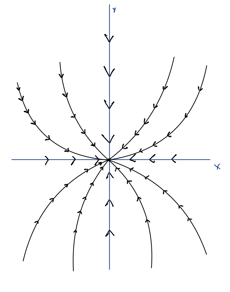
Example: Sink

$$A=\left[\begin{array}{cc}-1& 0\\ 0& -2\end{array}\right]$$

We find the following eigenvalues, with corresponding eigenvectors

$$\begin{array}{rlr}& \lambda =-1& \vec{v}=(1,0)\\ & \lambda =-2& \vec{v}=(0,1)\end{array}$$

For these eigenvectors, we see we have solutions

$$(1,0)e^{-t}(0,1)e^{-2t}$$

and thus, see that for any eigenvector (or multiple of an eigenvector), the orbits converge to the origin in a linear fashion as $t\to \infty$.

Furthermore, we see that these solutions form a general solution

$$x(t)=c_1{e}^{-t}y(t)=c_2{e}^{-2t}$$

and when $c_1,c_2\ne 0$, we obtain a point not on the axes. Noting that

$$y=\frac{c_2}{c_1^2}{x}^2$$

we see that as $t\to \infty$, all other orbits converge to the origin in a parabolic fashion!

Note that if our eigenvalues were flipped to be positive, we would have the exact same scenario, but with diverging orbits!
Also note that the parabolas asymptote towards the smaller eigenvalue!

Example: Saddle

$$A=\left[\begin{array}{cc}1& 0\\ 0& -2\end{array}\right]$$

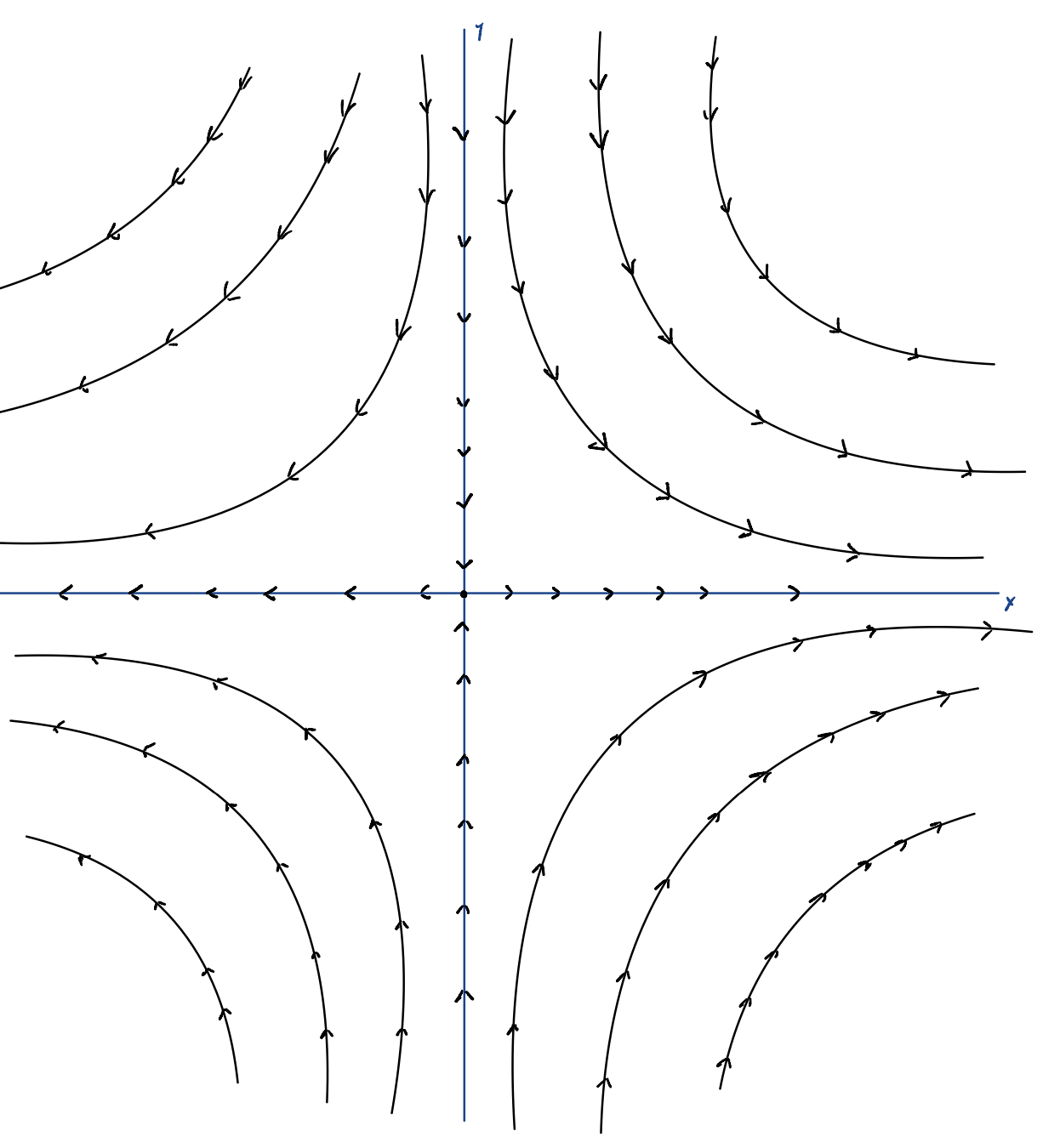
We find the following eigenvalues, with corresponding eigenvectors

$$\begin{array}{rlr}& \lambda =1& \vec{v}=(1,0)\\ & \lambda =-2& \vec{v}=(0,1)\end{array}$$

For these eigenvectors, we see we have solutions

$$(1,0)e^t(0,1)e^{-2t}$$

However, unlike the previous example, the orbits diverge along one eigenvector, yet converge along the other! So, our orbits follow the approximate paths:

Example: Circular Orbits

$$A=\left[\begin{array}{cc}0& 1\\ -1& 0\end{array}\right]$$

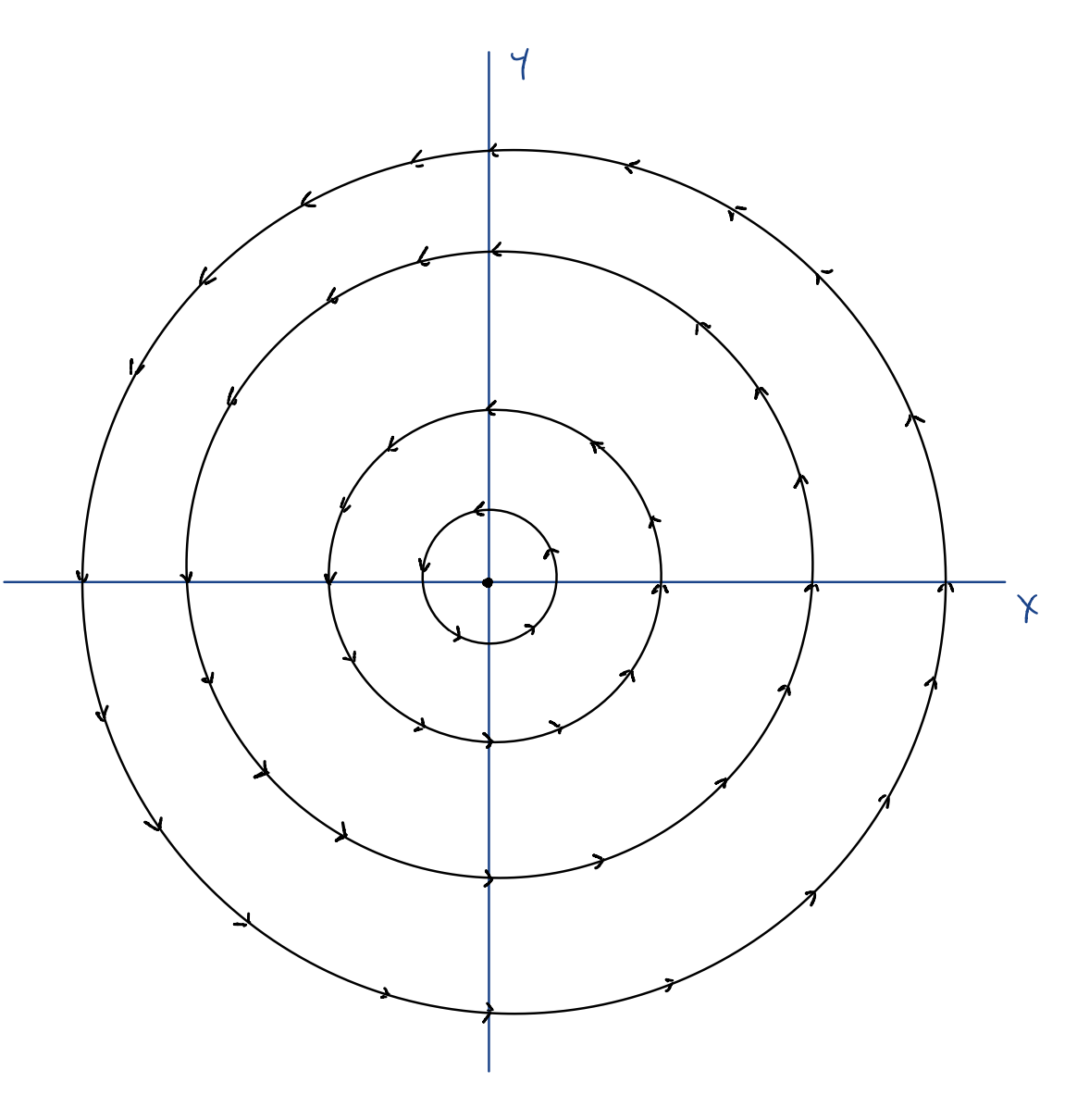
We find eigenvalues $\pm i$, giving us solutions $\cos (t)$ and $\sin (t)$.

Solving for the general solution, we find NFSoS to the respective linear differential equation

$$\begin{array}{rl}& N_0=\cos (t)\\ & N_1=\sin (t)\end{array}$$

and use it to find

$$e^{At}=I{N}_0+A{N}_1=\left[\begin{array}{cc}\cos (t)& \sin (t)\\ -\sin (t)& \cos (t)\end{array}\right]$$

which is actually the rotation matrix!

So, given any initial points $(c_1,c_2)$, we have an orbit given by solution

$$\left[\begin{array}{c}{c}_1\\ c_2\end{array}\right]\left[\begin{array}{cc}\cos (t)& \sin (t)\\ -\sin (t)& \cos (t)\end{array}\right]$$

in other words, all orbits are simply clockwise circular orbits of some radius about the origin.

Note that for matrix $A$ with purely imaginary eigenvalues, we would have similar results!

Example: Inward Spiral

$$A=\left[\begin{array}{cc}-1& 1\\ -1& -1\end{array}\right]$$

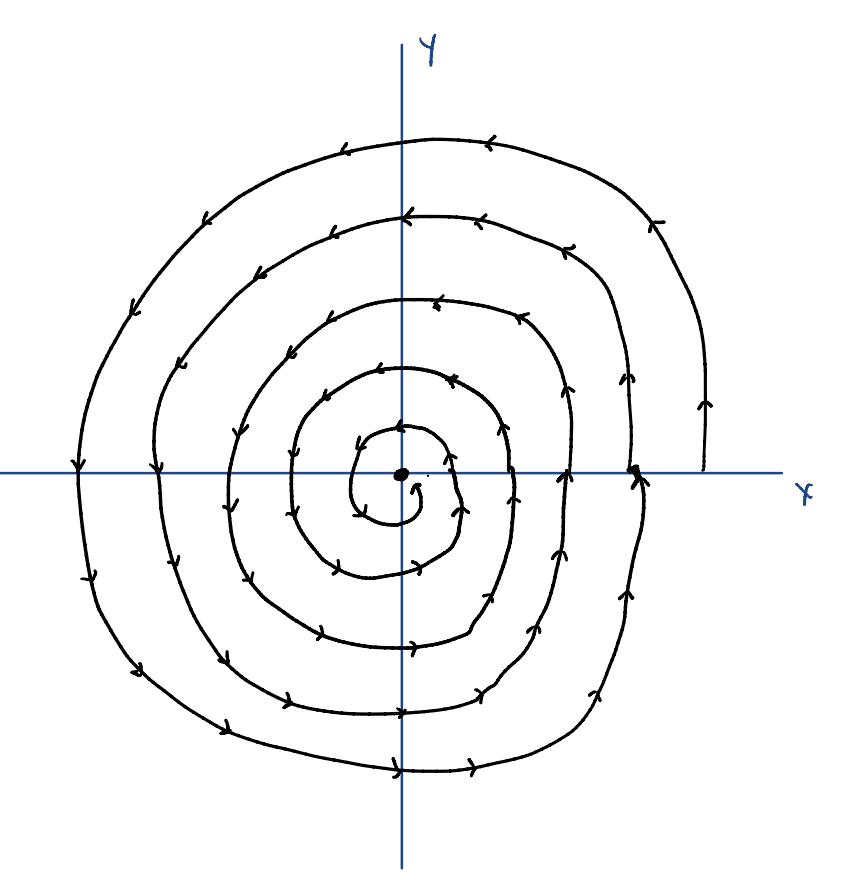
We find eigenvalues $-1\pm i$, giving us solutions $e^{-t}\cos (t)$ and $e^{-t}\sin (t)$. We use this to find a general solution

$$(\cos (t),-\sin (t))e^{-t}(\sin (t),\cos (t))e^{-t}$$

So, for any initial position $(c_1,c_2)$, we see that our orbit is a spiral inwards towards the origin!

Note that if the real part of our eigenvalues were positive, we would have had the exact opposite case - a spiral outwards!

In fact, from the above examples, we can note the following rules:

Theorem: Orbits and Linear Systems (2 Dimensional)

Say we have a linear system given by

$$\frac{d\vec{x}}{dt}=A\vec{x}$$

with characteristic polynomial $p(z)$. Let ${\lambda }_1$ and ${\lambda }_2$ be the eigenvalues for $A$, derived from $p(z)$. Then,

If ${\lambda }_1\ne {\lambda }_2$ are both real, and

• Both are positive, then the equilibrium is a source, and all orbits diverge parabolically (or linearly at the eigenvectors).
• Both are negative, then the equilibrium is a sink, and all orbits converge parabolically (or linearly at the eigenvectors).
• They are opposite signs, then the equilibrium is a saddle, and orbits converge along the negative eigenvalue, and diverge along the positive eigenvalue.

If ${\lambda }_1={\lambda }_2$ are both real, and

• $A$ is diagonalizable, then all solutions either converge (if negative) or diverge (if positive) from the origin linearly.
• $A$ is not diagonalizable, then all solutions either converge (if negative) or diverge (if positive) from the origin parabolically, along $A$‘s eigenvector.

If ${\lambda }_1,{\lambda }_2$ are imaginary with the form $a\pm bi$, and

• $a=0$, then all orbits are circles about the origin.
• $a<0$, then all orbits follow a stable (converging) spiral.
• $a>0$, then all orbits follow an unstable (diverging) spiral.

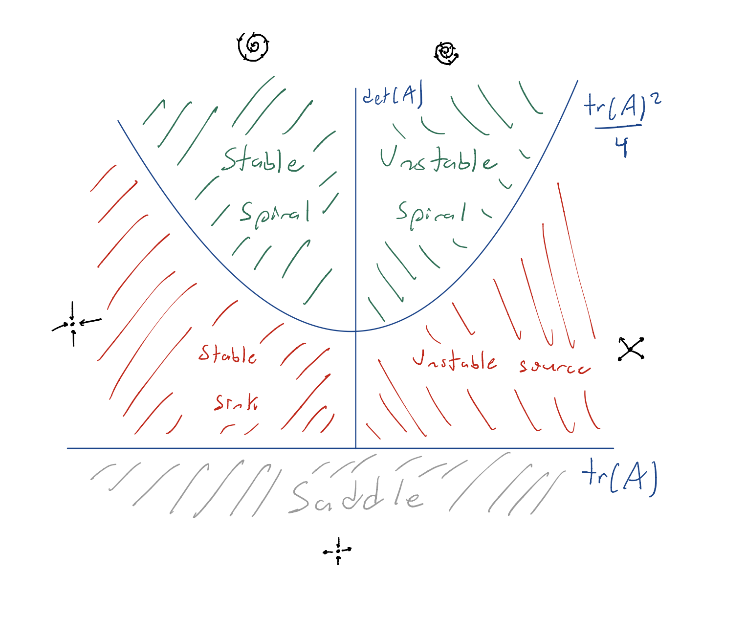
We use this theorem alongside the fact that the characteristic polynomial of a $2\times 2$ matrix can be given as

$$p(z)=z^2-tr(A)\cdot z+det(A)$$

where $tr(A)$ and $det(A)$ by the trace and determinant of $A$, respectively. This gives us roots (eigenvalues)

$$z=\frac{-tr(A)\pm \sqrt{tr(A{)}^2-4\cdot det(A)}}{2}$$

Then, if $det(A)\le \frac{tr(A{)}^2}{4}$, the eigenvalues are real, and

• If $det(A)<0$, the eigenvalues must have opposite signs.
• If $det(A)>0$, the eigenvalues have the same sign, and are negative if $tr(A)$ is negative, and positive if $tr(A)$ is positive.

Otherwise, if $det(A)>\frac{tr(A{)}^2}{4}$, the eigenvalues are complex, and can be expressed in the form $a\pm bi$.

We can use this fact, and trace a graph for $det(A)$ and $tr(A)$, with the behavior of orbits.

Orbits of Non-Linear Systems

Consider a non-linear differential system given by

$$\frac{d\vec{x}}{dt}=\vec{f}(\vec{x})$$

how can we determine the orbits of this differential system?

We can use what we know for linear systems! Given some equilibrium point, we can determine the behavior of orbits around that equilibrium, which can be merged (approximately) with the orbits of other equilibrium!

So, given a non-linear differential system, we want to

1. Find the equilibrium points
2. Linearize the system near these equilibrium points
3. Use this linearized system to trace the orbits

Let’s see an example below!

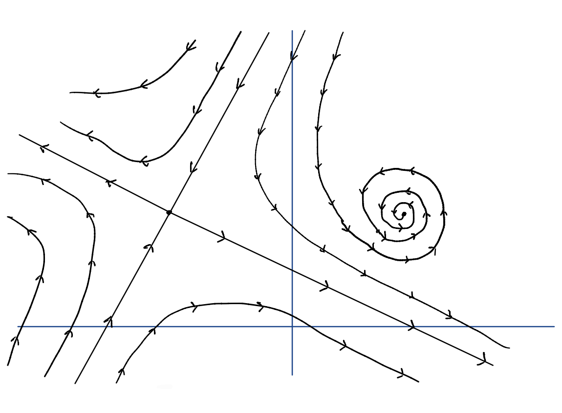
Example: Orbits and Non-Linear Systems

Suppose we have non-linear differential system

$$\frac{dx}{dt}=1-y\frac{dy}{dt}=x^2-y^2$$

Trace the orbits of the system.

To do this, we will first find our equilibrium points, by setting the derivatives to 0.

$$0=1-y0=x^2-y^2$$

We find points $y=1$, $x=\pm 1$.

Now, let’s linearize the system near these equilibrium points. We find Jacobian matrix

$$J=\left[\begin{array}{cc}{f}_x& f_y\\ g_x& g_y\end{array}\right]=\left[\begin{array}{cc}0& -1\\ 2x& -2y\end{array}\right]$$

and use this to linearize the system.

1. For $(1,1)$, we get Jacobian

   $$A=\left[\begin{array}{cc}0& -1\\ 2& -2\end{array}\right]$$

   Giving us eigenvalues $-1\pm i$, and because all eigenvalues are negative, points near the equilibrium take on some spiral inwards.

2. For $(-1,1)$, we find Jacobian

   $$A=\left[\begin{array}{cc}0& -1\\ -2& -2\end{array}\right]$$

   Giving us eigenvalues $-1\pm \sqrt{3}$, and because there is a positive and negative eigenvalue, the equilibrium point is a saddle.

We now find the eigenvectors to see where the orbits converge and diverge,

$$v_1=(1,2.73)v_2=(1,-0.73)$$

where orbits will converge along $v_1$, and diverge along $v_2$.

We use this to sketch a graph of the orbits! Note how the orbits will approximately take on the behavior of the equilibrium they are near.

Periodic Solutions

Limit Cycles

While we are interested in finding the orbits of an autonomous system, oftentimes we are interested in its closed orbits.

We define a limit cycle as an orbit of a periodic solution, taking on some simply closed curve (a closed curve that does not intersect itself).

Because the curve does not intersect itself, it has a defined tangent along every point!

Furthermore, a limit cycle is stable if points near it spiral towards the orbit. In other words, points inside the orbit should spiral outwards, and points outside the orbit should spiral inwards.

If only one spirals to the limit cycle while the other does not, it is semi-stable. Otherwise, it is unstable.

How do we know if a system does (and does not) have limit cycles?

Determining Limit Cycles

We will use vector fields to know if a system has (or does not have) limit cycles!

Given autonomous system

$$\frac{dx}{dt}=f(x,y)\frac{dy}{dt}=g(x,y)$$

we have a vector field $\vec{F}$, given by

$$\vec{F}=(f,g)=\left(\frac{dx}{dt},\frac{dy}{dt}\right)=\frac{dx}{dt}\hat{i}+\frac{dy}{dt}\hat{j}$$

tell us the velocity of the particle motion.

Given this vector field, we can prove the existence of a limit cycle using the following theorem:

Theorem: Poincare-Bendixson

Consider two simple closed curves, $C_1$ and $C_2$, where $C_2$ is enclosed by $C_1$. Define $R$ as the region between $C_1$ and $C_2$. Suppose $R$ contains no equilibrium points.

Let $\vec{F}=(f,g)$ be a vector field on ${\mathbb{R}}^2$. Then, if

1. On all points of the inwards curve $C_2$, $\vec{F}$ points outwards
2. On all points of the outwards curve $C_1$, $\vec{F}$ points inwards

there exists a limit cycle inside $R$.

Intuition $R$ has no equilibrium points, no points will ever stop inside $R$.

We know that because

Thus, if all points are pushed inwards from $C_1$, and outwards from $C_2$, there must necessarily be a curve where these “pushing forces” cancel one another out!

To prove a limit cycle, we find and explicitly show two curves $C_1$, $C_2$ satisfying this theorem!

Example: Proving Existence

Consider autonomous system given by

$$\frac{dx}{dt}=-y+x(1-x^2-y^2)\frac{dy}{dt}=x+y(1-x^2-y^2)$$

Prove there is a limit cycle in this system.

We find the vector field $\vec{F}$ as

$$\begin{array}{rl}& \vec{F}=f\hat{i}+g\hat{j}\\ & =(-y+x(1-x^2-y^2))\hat{i}+(x+y(1-x^2-y^2))\hat{j}\\ & =-y\hat{i}+x\hat{j}+x(1-r^2)\hat{i}+y(1-r^2)\hat{j}\\ & =(-y,x)+(x,y)(1-r^2)\end{array}$$

Now, observe that given position $\vec{P}=(x,y)$, we can find a tangent vector to the position as

$$\vec{T}=-y\vec{i}+x\vec{j}$$

Plugging this into our equation, we obtain

$$\vec{F}=\vec{T}+\vec{P}(1-r^2)$$

We use this equation to find the curves satisfying our theorem.

For $C_1$, let’s choose a circle of radius $r=2$. Then,

$$\vec{F}=T-3\vec{P}$$

so, along this entire circle, the vector field is pointing inwards!

For $C_2$, let’s choose a circle of radius $r=\frac{1}{2}$. Then,

$$\vec{F}=T+\frac{3}{4}\vec{P}$$

so, along this entire circle, the vector field is pointing outwards!

Finally, we see that in the region $\frac{1}{2}<r<2$, $\vec{F}$ is never 0, so there are no equilibrium points!

Thus, by the Poincare-Bendixson Theorem, we know in the region given by

$$\frac{1}{2}<r<2$$

there must exist a periodic solution.

Example: Proving Existence (2)

Consider autonomous system

$$\frac{dx}{dt}=y{e}^{1+x^2+y^2}\frac{dy}{dt}=-x{e}^{1+x^2+y^2}$$

We know our orbits are given as

$$\frac{dy}{dx}=\frac{g}{f}=-\frac{x}{y}\to x^2+y^2=C$$

they are circles!

Let’s see another way to determine if they are circular orbits.

Given a point $(x,y)$, we define its distance from the origin as

$$h(t)=x^2+y^2$$

taking its derivative, we obtain

$$\frac{dh}{dt}=2x\frac{dx}{dt}+2y\frac{dy}{dt}=2xy{e}^{1+x^2+y^2}-2xy{e}^{1+x^2+y^2}=0$$

so, our distance never changes!

Furthermore, as we see that $(0,0)$ is our only equilibrium point, it must be true that these curves are periodic solutions!

Alternatively, we can disprove the existence of a limit cycle using the following theorems.

Theorem: Bendixson-Criterion

Suppose region $D\subset {\mathbb{R}}^2$ is a closed bounded region which is simply connected.

Suppose $f_x+g_y$ is never 0 on $D$. Then, $D$ does not contain any closed orbits.

Proof $D$, which we'll name $C$.

Suppose by way of contradiction that we have a closed orbit in

Because $C$ is a closed curve, by Green’s theorem we know that

$$\oint (f\vec{i}+g\vec{j})\cdot \vec{n}ds=\iint \frac{\partial f}{dx}+\frac{\partial g}{dy}dxdy$$

Because $f_x$ and $g_y$ are never 0 on $D$, we know our integral is either always either positive or negative. But,

$$\oint (f\vec{i}+g\vec{j})\cdot \vec{n}ds$$

is always 0, as this integral is over the curve, giving us a contradiction!

Theorem: Closed Orbits and Equilibriums

Any closed orbit $C$ contains an equilibrium point in its interior.

Thus, if a closed region does not have any equilibrium points, there cannot be any closed orbits!

Example: Proving Nonexistence

Consider autonomous system given by

$$\frac{dx}{dt}=ax+by\frac{dy}{dt}=cx+dy$$

where $a,b,c,d$ are scalar values.

We know by the Bendixson-Criterion Theorem, if

$$f_x+g_y=a+d\ne 0$$

we have no periodic orbits!

Interestingly enough, as this is also a linear system, we find characteristic polynomial

$$p(z)=z^2-tr(A)z+det(A)$$

to find roots

$$z=\frac{tr(A{)}^2\pm \sqrt{tr(A{)}^2-4det(A)}}{2}$$

We know that if $tr(A)\ne 0$, we cannot have any periodic orbits, as there are no strictly imaginary eigenvalues! This agrees with our earlier finding!