Ordinary Differential Equations

An Ordinary Differential Equation is a rule relating derivatives of a function ($y$) on one variable ($t$).

Given an ordinary differential equation, our goal is to find the function(s) $y(t)$ satisfying the equation, known as solutions.

• A solution is a general solution if it represents all possible solutions to the system.
• A solution is a specific solution, if it is a solution to the system and satisfies some initial data provided, known as an initial value problem.

Here, we will discuss various methods and concepts surrounding solving ordinary differential equations!

First Order Differential Equations

A First Order Differential Equation is an ordinary differential equation whose highest order derivative is $y^{\prime }$.

All first order differential equations can be expressed in the form

$$\frac{dy}{dt}=f(t,y)$$

Where $f(t,y)$ is a function of $t$ and $y$.

Given a first order differential equation, we want to find the functions $y(t)$ satisfying the equation.

In an initial value problem to the equation, we want to find a solution satisfying $y(t_0)=y_0$, where $t_0,y_0\in \mathbb{R}$.

Explicit Equations

The Explicit First Order Differential Equation relates the derivative of $y$ to a function on $t$, as so:

$$\frac{dy}{dt}=f(t)$$

Where $f(t)$ is some function of $t$.

The explicit first order differential equation is arguably the easiest form of differential equation to solve! To solve, we simply take the antiderivative of both sides.

$$y(t)={\int }_{t_0}^{t}f(s)ds+C$$

Where $C$ is some arbitrary constant of integration.

Given initial value problem $y(t_0)=y_0$, we can solve for the specific solution by taking

$$y(t)=y_0+{\int }_{t_0}^{t}f(s)ds$$

As when $t=t_0$, the integral evaluates to 0, meeting the required conditions.

Example: Solving Explicit Equations

Find $y(t)$ such that

$$\frac{dy}{dt}=t^3-t$$

The domain of this differential equation is $\mathbb{R}$, the real number line. After integrating, we obtain

$$y(t)=\left(\frac{1}{4}{t}^4-\frac{1}{2}{t}^2\right)-\left(\frac{1}{4}{t}_0^4-\frac{1}{2}{t}_0^2\right)=\frac{1}{4}{t}^4-\frac{1}{2}{t}^2+C$$

Where $C$ represents some arbitrary constant.

This is the general solution to the differential equation.

The following theorem guarantees the existence of a solution for these equations.

Theorem: Existence and Uniqueness

Let $f:I\to \mathbb{R}$ be a continuous function, where $I$ is some interval.

For every $t_0\in I$, and any $y_0\in \mathbb{R}$, there exists a unique solution $y(t)$ defined on the same interval $I$, satisfying

$$\begin{array}{rl}{y}^{\prime }(t)& =f(t)\\ y(t_0)& =y_0\end{array}$$

Separable Equations

A separable equation is a differential equation which can be expressed in the form

$$g(y)\cdot \frac{dy}{dt}=f(t)$$

Where $g(y)$ and $f(t)$ are functions of $y$ and $t$, respectively.

We can easily solve this differential equation by integrating both sides with respect to their variables.

$$\int g(y)dy=\int f(t)dt$$

Example: Solving Separable Equations

Find the solutions of differential equation

$$y^{\prime }=2t{y}^2+3t^2{y}^2$$

We see that this differential equation is separable. Thus, we can integrate both sides with respect to their variables.

$$\begin{array}{rl}& y^{\prime }=2t{y}^2+3t^2{y}^2\\ & \frac{1}{y^2}{y}^{\prime }=2t+3t^2\\ & \int \frac{1}{y^2}dy=\int 2t+3t^{2}dt\\ & -\frac{1}{y}=t^2+t^3+C\\ & y=-\frac{1}{t^2+t^3+C}\end{array}$$

In some cases, a differential equation that isn’t separable can actually turn out to be.

For example, consider differential equation

$$\frac{dy}{dt}=\frac{y-t}{y+t}=\frac{\frac{y}{t}-1}{\frac{y}{t}+1}$$

Defining $u=y/t$, we find

$$y^{\prime }=u^{\prime }t+u\frac{dy}{dt}=\frac{u-1}{u+1}$$

Now, define function $h(u)$ as

$$h(u)=\frac{u-1}{u+1}$$

Then, we find

$$\begin{array}{rl}& u^{\prime }t+u=y^{\prime }=h(u)\\ & u^{\prime }=\frac{h(u)-u}{t}\end{array}$$

which is actually a separable equation!

Autonomous Equations

An autonomous equation is a separable equation in the form

$$y^{\prime }=g(y)$$

Where $g(y)$ is a function of $t$.

Notice how there is no explicit t-dependence provided.

Given an autonomous equation, we are commonly interested in its stationary solutions (discussed more in depth in Differential Systems).

We say solution $y(t)$ to a differential equation is stationary if

$$y(t)=c$$

Where $c$ is some constant value.

Also known as critical, fixed point, and equilibrium.

We can solve for stationary solutions from separable equations by solving for $g(y)=0$.

Linear First Order Equations

The Linear First Order Differential Equation follows the form

$$y^{\prime }+a(t)y=f(t)$$

Where $a(t)$ and $f(t)$ are functions of $t$.

Given a linear first order differential equation, the following theorem guarantees the existence of a solution.

Theorem: Existence and Uniqueness

Define linear first order differential equation

$$y^{\prime }+a(t)y=f(t)$$

Now suppose $f(t)$ and $a(t)$ are continuous on $I$.

Then, for some $t_0\in I$ and $y_0\in \mathbb{R}$, the initial value problem

$$\begin{array}{rl}{y}^{\prime }+a(t)y& =f(t)\\ y(t_0)& =y_0\end{array}$$

has a solution $y(t)$ on $I$.

Furthermore, this solution $y(t)$ is unique.

We now solve this differential equation.

General Solution

Take linear first order differential equation

$$y^{\prime }+a(t)y=f(t)$$

Define function $\mu (t)$, and multiply it with both sides of the equation.

Because we are multiplying both sides of the equation by the same function, we aren’t changing its solutions!

$$\mu (t)(y^{\prime }+a(t)y)=\mu (t)f(t)$$

Now, observe that

$$\frac{d}{dt}(\mu (t)y)=\mu (t)y^{\prime }+{\mu }^{\prime }(t)y$$

which is awfully similar to our differential equation! In fact, if we can find a function $\mu (t)$ such that ${\mu }^{\prime }(t)=\mu (t)a(t)$, then we can consolidate the left side of our equation to the above derivative.

We solve for a function $\mu (t)$ satisfying this property. Dividing by $\mu (t)$, we obtain

$$\frac{{\mu }^{\prime }(t)}{\mu (t)}=a(t)$$

Now, observe that

$$\frac{d}{dt}\ln (\mu (t))=\frac{{\mu }^{\prime }(t)}{\mu (t)}=a(t)$$

We can solve this to find $\mu (t)$ as

$$\mu (t)=e^{\int a(t)dt}=e^{A(t)}A(t)=\int a(t)dt$$

Plugging this back into our differential equation, we obtain

$$\begin{array}{rl}& \frac{d}{dt}(\mu (t)y)=\mu (t)y^{\prime }+{\mu }^{\prime }(t)y=\mu (t)f(t)\\ & \frac{d}{dt}(e^{A(t)}y)=e^{A(t)}f(t)\\ & y{e}^{A(t)}={\int }_{t_0}^{t}f(s)e^{A(s)}ds+C\\ & y=e^{-A(t)}\left({\int }_{t_0}^{t}f(s)e^{A(s)}ds+C\right)\end{array}$$

Where $A(t)=\int a(t)dt$, as our general solution to the linear equation.

Example: Solving Linear Equations

$$y^{\prime }+\cos (t)y=\cos (t)$$

We find $A(t)=\sin (t)$. Then

$$\begin{array}{rl}& \frac{d}{dt}{e}^{\sin (t)}y=e^{\sin (t)}\cos (t)\\ & e^{\sin (t)}y=e^{\sin (t)}+C\\ & y=1+C{e}^{-\sin (t)}\end{array}$$

Now suppose we have initial value problem $y(0)=5$. We can plug in to find $C=4$, to find our specific solution

$$y(t)=1+4e^{-\sin (t)}$$

Example: Long-Term Behavior of Linear Equations

Define the long-term behavior of linear equation

$$y^{\prime }+ay=a$$

defined on interval $I=(0,\infty )$, where $a\in \mathbb{R}$.

This differential equation defines a family of differential equations, because we can vary the $a$.

We solve the equation to find

$$y=1+C{e}^{-at}$$

We now describe the long behavior of this family through a case analysis.

• Case 1: For $a=0$, we find $y(t)=1+C$, a constant function.
• Case 2: For $a>0$, we find $y(t)=1+C{e}^{-at}$, which converges to $1$ as $t\to \infty$.
• Case 3: For $a<0$, we find $y(t)=a+C{e}^{at}$, which diverges as $t\to \infty$.

Exact Equations

Let $M(t,y)$ and $N(t,y)$ be functions on $t$ and $y$. Now, define differential equation

$$M(t,y)+N(t,y)y^{\prime }=0$$

This differential equation is exact, if there exists a function $\varphi (t,y)$ such that

$${\varphi }_t=M(t,y){\varphi }_y=N(t,y)$$

We can solve for $\varphi (t,y)$ by integrating $M(t,y)$ and $N(t,y)$ (shown below). We find a solution $\varphi (t,y)=c$, where to find a specific solution, we solve for $c$ given initial conditions $y_0$ and $t_0$.

This is a solution because we have eliminated the derivatives!

Theorem: Exact Differential Equations

Define differential equation

$$M(t,y)+N(t,y)y^{\prime }=0$$

where $M(t,y)$ and $N(t,y)$ are continuously differentiable on region $R$.

The differential equation is an exact differentiable exaction if and only if $M_y=N_t$ holds on all $R$.

We can connect this back to vector fields, and finding the potential function $f$ such that $\nabla f=\vec{F}$, where $\vec{F}$ is a conservative vector field.

Example: Solving Exact Equations

Determine if the following differential equation is exact.

$$e^{t}y+2t+(2y+e^t)y^{\prime }=0$$

We define

$$M=e^{t}y+2tN=2y+e^t$$

To determine if the differential equation is exact, we check $M_y=N_t$.

$$M_y=e^t=N_t$$

The equation is exact!

Let’s now solve for $\varphi (t,y)$.

$$\begin{array}{r}{\varphi }_t=M=e^{t}y+2t\to \\ \varphi =\int e^{t}y+2tdt=e^{t}y+t^2+g(y)\\ {\varphi }_y=e^t+g_y=N=2y+e^t\to \\ g_y=2y\to g=\int 2ydy=y^2+C\\ \varphi (t,y)=e^{t}y+t^2+y^2=C\end{array}$$

For any value $t$, $y$, we sub in to find $C$. That is our solution to the initial value problem.

Integrating Factor Technique

If the differential equation in the form

$$M(t,y)+N(t,y)y^{\prime }=0$$

is not exact, we may be able to make it exact by multiplying by function $\mu$, known as an integration factor.

$$\mu M(t,y)+\mu N(t,y)y^{\prime }=0$$

From before, to be exact, the following must hold true:

$$\begin{array}{rl}& (\mu M{)}_y=(\mu N{)}_t\\ & {\mu }_{y}M+u{M}_y=u_{t}N+\mu N_t\\ & \mu =\frac{{\mu }_{t}N-{\mu }_{y}M}{M_y-N_t}\end{array}$$

Solving for $\mu$ will yield us an integration factor to use to solve the equation.

The issue is, this differential equation for $\mu$ is a partial differential equation, which are notoriously difficult to solve.
Thus, we will look at unique cases where $\mu$ is independent of either $t$ or $y$. Which will simplify this equation so that we can solve for $\mu$.

1. Case 1: Suppose

   $$\frac{M_y-N_t}{N}=g(t)$$

   is independent of $y$ on $\mathbb{R}$. Then, we can find a $\mu$ such that $\mu$ is independent of $y$ (${\mu }_y=0$)! We sub this in and solve for ${\mu }_t$ as

   $${\mu }_t=\frac{M_y-N_t}{N}\mu =g(t)\mu$$

   We can then solve this differential equation to find $\mu$.

   $$\mu =e^{\int g(t)dt}$$

2. Case 2: Suppose

   $$f(y)=\frac{N_t-M_y}{M}$$

   is independent of $t$ on $\mathbb{R}$. Then, we can find a $\mu$ such that $\mu$ is independent of $t$ (${\mu }_t=0$)! We sub this in and solve for ${\mu }_y$ as

   $${\mu }_y=\frac{N_t-M_y}{M}\mu =f(y)\mu$$

   We can then solve this differential equation to find $\mu$.

   $$\mu =e^{\int f(y)dy}$$

Note: The integrating factor will not work when $\mu =0$, as this will yield a trivial solution which may not be present in the original differential equation.

Thus, the integrating factor will work best when the functions $M_y$ and $N_t$ are very different and do not equal each other much!

Example: Integrating Factor (1)

$$(2ty+2t^{2}y+y^2)+(t^2+y)y^{\prime }=0$$

We first observe that the equation is not exact.

$$M_y=2t+2t^2+2y\ne 2t=N_t$$

However, we find that

$$\frac{M_y-N_t}{N_t}=\frac{2t+2t^2+2y-2t}{t^2+y}=2$$

is independent of $y$! So, we can find an integrating factor $\mu$ independent of $y$ such that

$${\mu }_t=2\mu \to \mu =e^{2t}$$

We can now multiply our equation by our integrating factor, and solve!

Example: Integrating Factor (2)

$$y-t{y}^{\prime }=0$$

We first observe that the equation is not exact.

$$M_y=1\ne -1=N_t$$

However, we find that

$$\frac{N_t-M_y}{M}=\frac{-1-1}{y}=\frac{-2}{y}$$

So we can find an integrating factor $\mu$ independent of $t$ such that

$${\mu }_y=\frac{-2}{y}\mu \to \mu =y^{-2}$$

We can now multiply our equation by our integrating factor, and solve!

What if we cannot find $\mu$ independent of $t$ or $y$?
In this case, we try to find $\mu$ which takes a combination of $t$ and $y$ as an input, such as

$$\mu =f(t+y)$$

a single-variable function where the input is a combination of $t$ and $y$!

While this may seem like a convoluted approach, by the chain rule,

$${\mu }_y=f^{\prime }(t+y)(1){\mu }_t=f^{\prime }(t+y)(1)$$

Which, we can sub into the equation to obtain

$${\mu }_{y}M+u{M}_y=u_{t}N+\mu N_t$$ $$\to f^{\prime }M+f{M}_y=f^{\prime }N+f{N}_t$$

and eliminate the partial derivatives!

Example: Integrating Factor (Advanced)

$$2\sin (t)+(y+t)\cos (t)+2\sin (t)y^{\prime }=0$$

To solve this, take $\mu =f(t+y)$. We take the equation

\begin{align*} f' M + f M_y &= f' N + f N_t \\ &\to f' \cdot (2 \sin(t) + (y+t) \cos(t)) + f \cdot \cos(t) = f' \cdot 2 \sin(t) + f \cdot 2 \cos(t) \\ &\to f' (y + t) \cos(t) = f \cos(t) \\ &\to (y + t) f' = f \\

Letting $x=y+t$, we obtain the equation

$$x{f}^{\prime }(x)=f(x)$$

Which can be solved normally.

Well-Posed Equations

A differential equation is well-posed if:

1. It has a solution.
2. The solution is unique given initial conditions.
3. The solution depends continuously on initial data.

Only well-posed differential equations have predictive power, allowing us to use them in real-world applications (where many measurements are approximate).

Picard Iteration

Now consider a well-posed first order differential equation given by
$y^{\prime }(t)=f(t,y)$
where $f(t,y)$ is a function of $t$ and $y$, with known solution $y(t_0)=y_0$.

By integrating both sides of the differential equation, we obtain a new differential equation

$$\begin{array}{rl}& {\int }_{t_0}^t{y}^{\prime }(s)ds=y(t)-y(t_0)={\int }_{t_0}^{t}f(s,y)ds\\ & y(t)=y(t_0)+{\int }_{t_0}^{t}f(s,y)ds\end{array}$$

Because both differential equations have the same solutions, if we find a function $y(t)$ satisfying this equation, we will have found a solution to our original differential equation!

We want to find this function $y(t)$ that satisfies this differential equation!

Now say we have our known solution $y(t_0)=y_0$.

Using this solution, we can sub this into the equation to produce $y_1$, and then sub $y_1$ in to produce $y_2$, and so on and so forth. This can be described in the rule

$$y_{n+1}(t)=y_0+{\int }_{t_0}^{t}f(s,y_n(s))ds$$

These functions $y_n$ are successive approximations of $y(t)$, known as Picard Iterates.
If we can show that these Picard Iterates converge to a function on a suitable interval, we will have found our solution $y(t)$.

$$y(t)=\underset{n\to \infty }{\lim }{y}_n(t)$$

Remember that if we can find a single function $y(t)$ satisfying the differential equation, we will have found a solution to our original equation!

Example: Picard Iteration (1)

$$y^{\prime }=yy(0)=1$$

We solve this differential equation using Picard Iteration.

We now find our general formula for $y_n$ as

$$\begin{array}{rl}& y_{n+1}=y_0+{\int }_{t_0}^{t}f(s,y_n(s))ds\\ & y_{n+1}=1+{\int }_0^t{y}_n(s)ds\end{array}$$

Now, starting with our initial data, we continuously sub into our formula to find successive approximations of $y(t)$.

$$\begin{array}{rl}& y_0=1\\ & y_1=1+{\int }_0^{t}1ds=1+t\\ & y_2=1+{\int }_0^{t}1+tds=1+t+\frac{1}{2}{t}^2\\ & y_3=1+{\int }_0^{t}1+t+\frac{1}{2}{t}^{2}ds=1+t+\frac{1}{2}{t}^2+\frac{1}{3!}{t}^3\end{array}$$

Continuing this, we obtain the series

$$y_n=1+t+\frac{1}{2!}{t}^2+\frac{1}{3!}{t}^3+\cdots +\frac{1}{n!}{t}^n$$

Which converges to the function (and our solution)

$$y(t)=e^t$$

Example: Picard Iteration (2)

$$y^{\prime }=3yy(0)=1$$

We solve this differential equation using Picard Iteration.

We now find our general formula for $y_n$ as

$$\begin{array}{rl}& y_{n+1}=y_0+{\int }_{t_0}^{t}f(s,y_n(s))ds\\ & y_{n+1}=1+{\int }_0^{t}3y_n(s)ds\end{array}$$

Now, starting with our initial data, we continuously sub into our formula to find successive approximations of $y(t)$.

$$\begin{array}{rl}& y_0=1\\ & y_1=1+{\int }_0^{t}3(1)ds=1+3t\\ & y_2=1+{\int }_0^{t}3(1+3t)ds=1+3t+\frac{3^2}{2}{t}^2\\ & y_3=1+{\int }_0^{t}3(1+3t+\frac{3^2}{2}{t}^2)ds=1+3t+\frac{3^2}{2}{t}^2+\frac{3^3}{3!}{t}^3\end{array}$$

Continuing this, we obtain the series

$$y_n=1+3t+\frac{3^2}{2}{t}^2+\frac{3^3}{3!}{t}^3+\cdots +\frac{3^n}{n!}{t}^n$$

Which converges to the function (and our solution)

$$y(t)=e^{3t}$$

Convergence of Picard Iterates

Performing Picard Iteration on nonlinear differential equations may fail, as solutions of nonlinear differential equations may not exist for all time $t$. Thus, the Picard iterates will similarly fail to converge for all $t$.

The following theorem helps us find an interval where all $y_n(t)$ are bounded ($y_n(t)\le K,K\in \mathbb{R}$), and provide a rectangle where all these iterates $y_n$ exist.

Theorem: Picard–Lindelöf

Let $a,b\in \mathbb{R}$. Choose $R$ as the rectangle bounded by

$$t_0\le t\le t_0+a|y-y_0|\le b$$

Let $f$ be differentiable, and $\frac{\partial f}{\partial y}$ be continuous in $R$.

We define $M$ as the maximum of $f(t,y)$ in $R$, and $\alpha$ as the following:

$$M=\underset{R}{\max }|f(t,y)|\alpha =\min \left(a,\frac{b}{M}\right)$$

Then, for every $t$ in the interval $t_0\le t\le t_0+\alpha$, the Picard iterates must be contained in $R$, and moreover, will converge.

The theorem shows $y_n(t)$ must necessarily be sandwiched between the lines

$$y=y_0+M(t-t_0)y=y_0-M(t-t_0)$$

For $t_0\le t\le t_0+\alpha$, which exit the rectangle at either $a$ or $\frac{b}{M}$ (whichever comes first).

Then, there exists a unique solution $y(t$) defined on the interval $[t_0,t_0+\alpha ]$ for the initial value problem

$$y^{\prime }=f(t,y)y(t_0)=y_0$$

Furthermore, $|y(t)-y(t_0)|\le b$ along this interval.

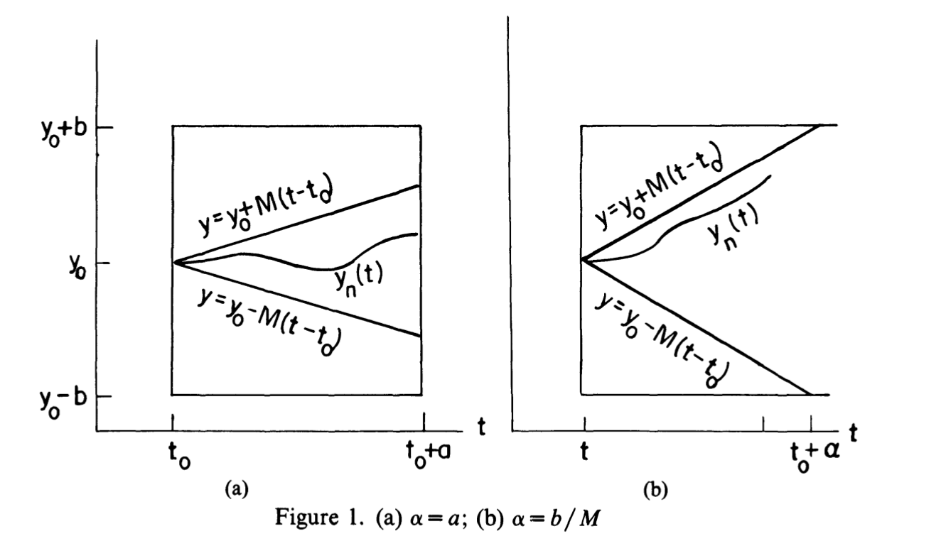
It’s important to note that this theorem only allows us to make local approximations. Increasing the size of $R$ will also increase $M$ in size, eventually limiting our interval of approximation.

Example: Existence of Picard Iterates

Show that the solution $y(t)$ to the IVP

$$\frac{dy}{dt}=e^{-t^2}+y^{3}y(0)=1$$

Exists for $0\le t\le \frac{1}{9}$, and in this interval, $0\le y\le 2$.

Let $R$ be the rectangle bounded by

$$0\le t\le \frac{1}{9}0\le y\le 2$$

We compute $M$ as

$$M=\underset{R}{\max }(e^{-t^2}+y^3)=e^0+2^3=9$$

And see that $y(t)$ exists for

$$\begin{array}{r}\alpha =\min \left(\frac{1}{9},\frac{1}{9}\right)=\frac{1}{9}\\ t_0=0\le t\le t_0+\alpha =\frac{1}{9}\\ 0\le t\le \frac{1}{9}\end{array}$$

And in this interval, $0\le y\le 2$.

Example: Existence of Picard Iterates (2)

$$y^{\prime }=yy(1)=e$$

Lets choose $R$ as the rectangle bounded by

$$1\le t\le 3y-y_0\le b$$

Then, we find

$$M=\underset{R}{\max }|y|=e+b\alpha =\min \left(2,\frac{b}{e+b}\right)=\left(2,1-\frac{e}{e+b}\right)$$

Letting $b\to \infty$, we observe that $\alpha$ converges to 1 to yield an interval of $[1,2)$ which the approximation exists on.

Example: Existence of Picard Iterates (3)

$$y^{\prime }=e^{-y^2}+e^{-t}y(0)=2$$

Define $R$ as the region where $t\ge 0$.

We find $M$ and $\alpha$ to be

$$M=\underset{R}{\max }|e^{-y^2}+e^{-t}|\le e^0+e^0=2$$ $$\to \alpha =\min \left(a,\frac{b}{2}\right)$$

Letting $b=2a$, we obtain $\alpha =a$, creating an interval of $[0,a]$. Because there is no bound on $a$, we have proven that there exists a solution for all $y(t)$, $t>0$.

Higher Order (Linear) Differential Equations

We now begin our discussion of higher order ordinary differential equations.

For simplicity, when dealing with the higher order, we will only deal with linear differential equations, defined later.

Linear Differential Equations

Given some differential equation, we define it as linear if all functions $y$ and its derivatives are all in the first power, and are independent of one another.

We define the order of a linear differential equation as the degree of its highest derivative.

Given any $n^{th}$ order linear differential equation, we can express it in the form

$$\frac{d^{n}y}{d{t}^n}+a_n(t)\frac{d^{n-1}y}{d{t}^{n-1}}+\cdots +a_2(t)\frac{dy}{dt}+a_1(t)y=f(t)$$ $$\to y^n+a_n(t)y^{n-1}+\cdots +a_2(t)y^1+a_1(t)y=f(t)$$

known as the equation’s standard (normal) form.

Note: All coefficients and $f(t)$ are functions of $t$.

We call $f(t)$ the forcing equation, as it sets a constraint which all solutions $y(t)$ must follow. When $f(t)=0$, the equation is homogeneous.
Otherwise, when $f(t)\ne 0$, the equation is non-homogeneous.

Now define $D=\frac{d}{dt}$ as the derivative operator. Using $D$, we can redefine the differential equation as

$$L[y]=f(t)$$

Where $L$ is the $n^{th}$ order linear operator defined by

$$L=D^n+a_n(t)D^{n-1}+\cdots +a_2(t)D+a_1(t)$$

We commonly represent differential equations using this operator!

It may sometimes help to think of $L$ as a linear map from $n$ differential functions to continuous functions.

$$L:C^n(I)\to C^0(I)$$

Properties of Solutions

When given a differential equation, often our primary goal is to solve it, or in other words, find all functions $y(t)$ satisfying the equation. In other words, a function $y_0$ is a solution to the differential equation if

$$L[y_0]=f(t)$$

Now suppose we have some homogeneous $n^{th}$ order linear equation given by

$$L[y]=0$$

Then, given any two solutions to this equation $y_1$ and $y_2$, we see that by property of linear operators,

$$\begin{array}{rl}& L[y_1+y_2]=L[y_1]+L[y_2]=0\\ & L[c\cdot y_1]=cL[y_1]=0\end{array}$$

So, we can form new solutions to our differential equation using combinations of known solutions! This forms a space of solutions, described in the following theorem.

Theorem: Solutions to Homogenous Equations

Suppose we have homogenous $n^{th}$ order differential equation

$$L[y]=0$$

where $L$ is the linear operator given by

$$L=D^n+a_n(t)D^{n-1}+\cdots +a_2(t)D+a_1(t)$$

Then, the set of solutions to the homogeneous equation is a vector space $V$ with $dim(n)$, where $V\subset C^n$, the set of all functions differentiable (at least) $n$ times.

Furthermore, $V=ker(L)$.

Now, given a non-homogeneous equation

$$L[y]=f(t)$$

with known solution $y_P$, and solution to corresponding homogeneous equation $y_H$, note that we can form new solutions to the non-homogeneous equation by combining these two solutions!

$$L[y_P+y_H]=L[y_P]+L[y_H]=f(t)+0=f(t)$$

This is formalized in the following theorem.

Theorem: Solutions for Homogenous and Non-Homogenous Equations

Suppose we have a non-homogenous differential equation

$$L[y]=f(t)$$

with some known solution $y_P(t)$.

Then, the general solution to this non-homogenous differential equation is

$$y(t)=y_H(t)+y_P(t)$$

Where $y_H(t)$ is the general solution to the associated homogenous differential equation $Ly=0$.

Alternatively, we can find a single function $y(t)$, or set of functions in the solution set, satisfying an Initial Value Problem (IVP). In these problems, we’re given initial conditions

$$\begin{array}{rl}y(t_0)& =y_0\\ y^{\prime }(t_0)& =y_1\\ & ⋮\\ y^{n-1}(t_0)& =y_{n-1}\end{array}$$

And are tasked with finding a solution to the differential equation $y(t)$, which also satisfies these conditions at $t_0$.

Typically, all of the initial conditions will be given in terms of one point $t=t_0$, as this is the most practical use of initial value problems.

Fundamental Sets of Solutions

Let $L[y]=f(t)$ be a differential equation, and suppose $V$ is the set of all solutions to this differential equation.

Now suppose we have a set of solutions $S=\{y_1(t),y_2(t),\dots ,y_n(t)\}$. We say this set forms a Fundamental Set of Solutions (FSoS) for the differential equation if it is a basis of $V$. In other words, the set:

• Is Linearly Independent: No functions in the set can be recreated as scalar combinations of the others.
• Spans $V$: All solutions in $V$ can be created as a combination of the functions in this set.

Now suppose we have a point $t_0\in I$.
Define a fundamental set of solutions $\{N_0(t),\dots ,N_{n-1}(t)\}$. We say this set is a Natural Fundamental Set of Solutions (NFSoS) if

$$\begin{array}{cccc}{N}_0(t_0)=1& N_1(t_0)=0& \dots & N_{n-1}(t_0)=0\\ N_0^1(t_0)=0& N_1^1(t_0)=1& \dots & N_{n-1}^1(t_0)=0\\ N_0^2(t_0)=0& N_1^2(t_0)=0& \dots & N_{n-1}^2(t_0)=0\\ ⋮& ⋮& & ⋮\\ N_0^{n-1}(t_0)=0& N_1^{n-1}(t_0)=0& \dots & N_{n-1}^{n-1}(t_0)=1\end{array}$$

In other words, all $N_i$ at $t_0$ are 1 only on their $i^{th}$ derivative, and 0 for all other derivatives. This is a fundamental set of solutions that’s very “nice” to use at the IVP $t=t_0$.

Solving Initial Value Problems with the NFSoS

Why are we interested in the Natural Fundamental Set of Solutions?

Let $\{N_0(t),\dots ,N_{n-1}(t)\}$ be a NFSoS at $t=t_0$ to the differential equation $L[y]=f(t)$. By definition, all solutions to the differential equation can be expressed in terms of these functions.

In other words, for any arbitrary solution $y(t)$,

$$y(t)=c_0{N}_0(t)+c_1{N}_1(t)+\cdots +c_{n-1}{N}_{n-1}(t)$$

Now consider initial value problem at $t=t_0$ such that

$$y(t_0)=y_0{y}^1(t_0)=y_1\dots y^{n-1}(t_0)=y_{n-1}$$

We observe that by definition of a NFSoS, at various derivatives of $y(t)$ at $t=t_0$,

$$\begin{array}{rl}& y(t_0)=y_0=c_0{N}_0(t_0)+0+\cdots +0=c_0\\ & y^1(t_0)=y_1=0+c_1{N}_1(t_0)+0+\cdots +0=c_1\\ & ⋮\\ & y^i(t_0)=y_i=c_i\\ & ⋮\\ & y^{n-1}(t_0)=y_{n-1}=c_{n-1}{N}_{n-1}(t_0)=c_{n-1}\end{array}$$

Thus, for any initial conditions $y_0,y_1,\dots ,y_{n-1}$, we can easily find the solution to the IVP as

$$y(t)=y_0{N}_0(t)+y_1{N}_1(t)+\cdots +y_{n-1}{N}_{n-1}$$

Example: Fundamental Set of Solutions

Take differential equation

$$y^{\prime \prime }-5y^{\prime }+6y=0$$

We see that $L=D^2-5D+6I$.

We can find the basis for the set of solutions $V$ as $\{e^{2t},e^{3t}\}$. So, all solutions for the differential equation can be represented in the general form

$$y=c_1{e}^{2t}+c_2{e}^{3t}$$

Where $c_1,c_2$ are scalar values.

Now, say we want to find the fundamental set of solutions at $t_0=0$ such that

$$N_0(0)=1N_0^{\prime }(0)=0$$ $$N_1(0)=0N_1^{\prime }(0)=1$$

We find these as $N_0=3e^{2t}-2e^{3t}$, and $N_1=e^{3t}-e^{2t}$. This fundamental set of solutions is highly useful , as if we have some initial value problem

$$y(0)=y_0{y}^{\prime }(0)=y_1$$

We can easily find the solution as

$$y(t)=y_0{N}_0(t)+y_1{N}_1(t)$$

The Wronskian

How do we know if our set of solutions is a fundamental set of solutions?

Suppose we have differential equation $L[y]=f(t)$, with $V$ representing the set of all solutions.
Now suppose we have a set of solutions $S=\{g_1,\dots ,g_n\}$. We know $S$ is a basis if $\forall t_0\in I$ and all initial conditions $y_0,y_1,\dots ,y_{n-1}$, we can find scalars $c_1,c_2,\dots ,c_n$ such that the solution $y(t)$ can be uniquely expressed as a combination of the functions in $S$.

$$y(t)=\sum _{i=1}^n{c}_i{g}_i(t)$$

In other words, the set on $n$ elements spans the solution set.

Say we have initial conditions $y_1,y_2,\dots ,y_n$ at $t=t_0$, and let $c_1,c_2,\dots ,c_n$ be scalars.
Then, our set of functions must satisfy

$$\begin{array}{rl}& c_1{g}_1(t_0)+c_2{g}_2(t_0)+\cdots +c_n{g}_n(t_0)=y_1\\ & c_1{g}_1^1(t_0)+c_2{g}_2^1(t_0)+\cdots +c_n{g}_n^1(t_0)=y_2\\ & c_1{g}_1^2(t_0)+c_2{g}_2^2(t_0)+\cdots +c_n{g}_n^2(t_0)=y_3\\ & ⋮\\ & c_1{g}_1^{n-1}(t_0)+c_2{g}_2^{n-1}(t_0)+\cdots +c_n{g}_n^{n-1}(t_0)=y_n\end{array}$$

Which is a system of equations, which can be represented in matrix form

$$\left[\begin{array}{cccc}{g}_1(t_0)& g_2(t_0)& \dots & g_n(t_0)\\ g_1^1(t_0)& g_2^1(t_0)& \dots & g_n^1(t_0)\\ ⋮& ⋮& \ddots & ⋮\\ g_1^{n-1}(t_0)& g_2^{n-1}(t_0)& \dots & g_n^{n-1}(t_0)\end{array}\right]\left[\begin{array}{c}{c}_1\\ c_2\\ ⋮\\ c_n\end{array}\right]=\left[\begin{array}{c}{y}_1\\ y_2\\ ⋮\\ y_n\end{array}\right]$$

To uniquely satisfy this system of equations, the $g$ matrix must be invertible. Thus, by the invertible matrix theorem, the determinant of the matrix cannot be 0!

Let $\{h_1,\dots ,h_n\}$ be a set of solutions to some differential equation.
We define the Wronskian, denoted $W(h_1,\dots ,h_n)$ as

$$W=det\left(\left[\begin{array}{ccccc}{h}_1& h_2& h_3& \dots & h_n\\ h_1^1& h_2^1& h_3^1& \dots & h_n^1\\ h_1^2& h_2^2& h_3^2& \dots & h_n^2\\ ⋮& ⋮& ⋮& \ddots & ⋮\\ h_1^n& h_2^n& h_3^n& \dots & h_n^n\end{array}\right]\right)$$

If the set of solutions is a fundamental set of solutions, the Wronskian cannot be 0 for any $t_0\in I$ on which the differential equation is defined!

This is because by taking the Wronskian, we are simultaneously evaluating invertibility for all $t$, and if there is any $t$ making the determinant 0, the functions are not linearly independent for that $t$!

Theorem: Wronskian and FSoS

Suppose we have a differential equation

$$y^n+a_n(t)y^{n-1}+\cdots +a_2(t)y^1+a_1(t)y=f(t)$$

Defined on $I=(a,b)\subseteq \mathbb{R}$.

Let $\{g_1,\dots ,g_n\}$ be a set of solutions to the differential equation. These functions are a fundamental set of solutions to the differential equation if the Wronskian $W\ne 0$ for all $t_0\in I$.

$$W(g_1,\dots ,g_n)\ne 0$$

The following theorem simplifies this fact - it guarantees that if we find $t_0\ne 0$ for any $t_0\in I$, the Wronskian is never 0 on which $I$ is defined!

So, if the Wronskian $W\ne 0$ for any $t_0$, we know that our set of functions is a fundamental set of solutions!

Theorem: Abel's Theorem

Suppose we have homogeneous $n^{th}$ order linear differential equation of the form

$$y^n+p_{n-1}{y}^{n-1}+\cdots +p_1{y}^{\prime }+p_{0}y=0$$

defined over interval $I$. Then, the Wronskian of any fundamental set of solutions $W(y_1,y_2,\dots ,y_n)$ must satisfy the relationship

$$W^{\prime }+p_{n-1}W=0$$

Furthermore, by solving for the Wronskian, we can find it as

$$W(y_1,y_2)=C{e}^{\int -p_{n-1}dt}$$

Corollary: By this theorem, we see that the Wronskian is always positive, always 0, or always negative over $I$, for any $n^{th}$ order homogeneous linear differential equation.

This theorem (and corollary) can be generalized to higher order equations.

Proof

Suppose we have two solutions to the differential equation $\{y_1,y_2\}$. We that by definition, the Wronskian is given by

$$W(y_1,y_2)=y_1{y}_2^{\prime }-y_2{y}_1^{\prime }$$

We then calculate the derivative of the Wronskian as follows:

W' = y_1' y_2' + y_1 y_2'' - y_2' y_1' - y_2 y_1'' = y_1 y_2'' - y_2 y_1'' $$ Now take differential equation

y” + p(t) y’ + q(t) y = 0

Because we know that $y_1$ and $y_2$ are, by definition, solutions to the differential equation,

\begin{align*}
&y_1” + p(t) y_1’ + q(t) y_1 = 0 \
&y_2” + p(t) y_2’ + q(t) y_2 = 0
\end{align*}

Multiplying the first equation by $-y_2$, and the second by $y_1$ and adding the two equations together, we obtain

\begin{align*}
-&y_2 y_1” - p(t) y_2 y_1’ - q(t) y_2 y_1 = 0 \
&y_1 y_2” + p(t) y_1 y_2’ + q(t) y_1 y_2 = 0 \
&(y_1 y_2” - y_2 y_1”) + p(t) (y_1 y_2’ - y_2 y_1’) = 0 \
&W’ + p(t) W = 0
\end{align*}

$$WecanthenusethistofindtheWronskianas$$

\frac{W’}{W} = -p(t) \to \ln(W) = \int -p(t) dt + C

W = C e^{\int -p(t) dt}

We now discuss finding solutions to these higher order differential equations.

Constant Homogeneous Equations

We define a constant differential equation as an $n^{th}$ order differential equation $L[y]=f(t)$

$$y^n+a_n(t)y^{n-1}+\cdots +a_2(t)y^1+a_1(t)y=f(t)$$

such that $a_1(t),a_2(t),\dots ,a_n(t)$ are all constants, and $f(t)$ is a function on $t$.

In this section, we discuss how we solve the constant homogeneous differential equation

$$y^n+a_n(t)y^{n-1}+\cdots +a_2(t)y^1+a_1(t)y=0$$

and later use these findings to solve the non-homogeneous variant.

2nd Order Case

Consider the $2^{nd}$ order case

$$y^{\prime }+ay=0$$

We want to find solutions $y(t)$ to this differential equation. In other words, we want to find

$$L[y]=0$$

Where $L=D+aI$.

We can easily find the general solution as $y(t)=C{e}^{-at}$, where $C$ is some scalar, giving us a solution set of $span\{e^{-at}\}$.

Example: Homogeneous Second Order Cases

Let $L$ be the linear operator to some homogeneous constant differential equation. Then,

• If $L=D-3I$, we have solution $e^{3t}$.
• If $L=D-5I$, we have solution $e^{5t}$.

Higher Order Cases

Now let’s consider higher order cases. Given some new linear operator $L$, we can express the higher order cases as a composition of $2^{nd}$ order cases.

For example,

$$L=(D^2-8D+15I)=(D-3I)(D-5I)=(D-5I)(D-3I)$$

Let $M=(D-3I)$ and $N=D-5I$ be $2^{nd}$ order linear operators. Then,

$$L[y]=MN[y]=NM[y]=0$$

Now say we have a solution $y(t)$ to the differential equation $L[y]=0$. Then, $y(t)$ just needs to satisfy $M[y]=0$ or $N[y]=0$. Thus, we find the solution set to be $\{e^{3t},e^{5t}\}$.

Notice how our solutions to the higher order differential equation are the solutions to each 2nd order “root”.

We can generalize from this example for any number of roots.

Theorem: Solutions to Homogenous Equations with Constant Coefficients

Let $L$ be a linear operator with constant coefficients $a_1,a_2,\dots ,a_n$

$$L=D^n+a_n{D}^{n-1}+\cdots +a_{2}D+a_{1}I$$

and let $p(z)$ be the characteristic polynomial of $L$ such that

$$p(z)=z^n+a_n{z}^{n-1}+\cdots +a_{n}z+a_1$$

with distinct roots $z_1,\dots ,z_n\in \mathbb{C}$.

Then, the fundamental set of solutions for homogenous $n^{th}$ order differential equation represented by $L$

$$L[y]=0$$

is $\text{FSoS}=\{e^{z_{1}t},e^{z_{2}t},\dots ,e^{z_{n}t}\}$.

Solutions with Complex Roots

Say $a\pm bi$ is a pair of complex roots to $p(z)$. Then the complex solutions corresponding to the conjugate pairs $e^{(a+bi)t},e^{(a-bi)t}$ can be replaced by real solutions

$$e^{at}\cos (bt),e^{at}\sin (bt)$$

These real functions are much more useful in real world applications!

A simple proof for this is given below.

Proof

Say we have solutions $e^{(a\pm bi)t}$. Then,

e^{(a \pm bi) t} = e^{at} e^{\pm ibt} = e^{at} ( \cos(bt) \pm i \sin(bt) )

\to { e^{at} \cos(bt), e^{at} \sin(bt) }

Example: Solving Constant Homogenous Differential Equations

Suppose we have differential equation given by

$$y^{\prime \prime }-7y^{\prime }+10y=0$$

We obtain the characteristic polynomial for the equation as

$$p(z)=z^2-7z+10=(z-5)(z-2)=0$$

To obtain solution set $\{e^{2t},e^{5t}\}$.

We then show it is a fundamental set of solutions by finding the Wronskian.

$$W(e^{2t},e^{5t})=3e^{7t}\ne 0$$

Repeated Roots

Suppose $p(z)$ has a repeated root $a$ with multiplicity $m$.

Multiplicity of Roots

Say $z=c$ is a root of $p(z)$. Then, the multiplicity of $c$ as a root of $p(z)$ is $m$ if and only if

$$p(z)=0,p^{\prime }(z)=0,\dots p^{m-1}(z)=0,p^m(z)\ne 0$$

Corollary: $p(z)$ has a repeated root if and only if it shares a root with its derivatives.

As shown earlier, we know that $e^{at}$ is a solution to the differential equation. Now, observe that

$$\begin{array}{rl}& (D-aI)e^{at}=0\\ & (D-aI{)}^{2}t{e}^{at}=(D-aI)e^{at}=0\\ & (D-aI{)}^3{t}^2{e}^{at}=(D-aI{)}^{2}t{e}^{at}=(D-aI)e^{at}=0\\ & ⋮\end{array}$$

Thus, we see that the repeated root $a$ has solution set $\{1e^{at},t{e}^{at},\dots ,t^{m-1}{e}^{at}\}$.

This is very similar to generalized eigenvectors in Jordan form!

We additionally show that this set is linearly independent.
Define $T:C^0(\mathbb{R})\to C^0(\mathbb{R})$ as a linear transformation such that $T(f(t))=f(t)e^{at}$.
We see that $ker(T)=\{0\}$. Then, taking linear combination

$$c_1{e}^{at}+c^{2}t{e}^{at}+\cdots +c_n{t}^{n-1}{e}^{at}=0$$ $$\to T(c_1+c_{2}t+\cdots +c_n{t}^{n-1})=0$$

As the kernel of $T$ is 0, all coefficients are forced to be 0.

Solutions with Repeated Roots

Let $L$ be a linear operator with constant coefficients $a_1,a_2,\dots ,a_n$

$$L=D^n+a_n{D}^{n-1}+\cdots +a_{2}D+a_{1}I$$

and let $p(z)$ be the characteristic polynomial of $L$ such that

$$p(z)=z^n+a_n{z}^{n-1}+\cdots +a_{n}z+a_1$$

Suppose $c$ is a root of $p(z)$ with multiplicity $m$. Then, the solution set to this root $c$ is given by $\{1e^{ct},t{e}^{ct},\dots ,t^{m-1}{e}^{ct}\}$.

Example: Solving Constant Homogenous Equations (1)

Suppose we have differential equation with characteristic polynomial given by

$$p(z)=(z-5{)}^4(z-3)(z+7{)}^2$$

Then, the set of solutions for the differential equation is given by

$$\{e^{5t},t{e}^{5t},t^2{e}^{5t},t^3{e}^{5t},e^{3t},e^{-7t},t{e}^{-7t}\}$$

We then show that this set of functions is linearly independent (using the Wronskian) to show that it is a fundamental set of solutions.

Example: Solving Constant Homogenous Equations (2)

$$p(z)=(z-(3+4i){)}^2(z-5{)}^3(z+(3+4i){)}^2$$

Has solution set

$$\{e^{5t},t{e}^{5t},t^2{e}^{5t},e^{3t}\cos 4t,t{e}^{3t}\cos 4t,e^{3t}\sin 4t,t{e}^{3t}\sin 4t\}$$

Example: Finding Periodic Solutions

Suppose we have differential equation

$$y^4-y=0$$

What are the differential equation’s periodic solutions?

We find the characteristic polynomial as $p(z)=z^3(z-1)$, yielding roots $\pm 1,\pm i$ and solution set

$$\{e^t,e^{-t},e^{\pm it}\}$$

Inspecting the solution set, we see that we have periodic solutions $e^{\pm it}=\{c_1\cos (t),c_2\sin (t)\}$, where $c_1,c_2$ are some scalar value.

Constant Non-Homogeneous Equations

Now say we have a constant non-homogeneous differential equation

$$L[y]=f$$

Where $f$ is some constant value.

How can we find this equation’s fundamental set of solutions?

By an earlier theorem, we know that if we have the general solution set to the associated homogeneous differential equation

$$L[y]=0$$

and a specific solution $y_p$ to the non-homogeneous differential equation, then all solutions of $L[y]=f$ can be found as

$$y(t)=y_H+y_p$$

Where $y_H$ is the general solution to the homogeneous differential equation.

This is because, by property of linear transformations,

$$L[y_H+y_p]=L[y_H]+L[y_p]=0+f$$

Telling us that $y_H+y_p$ is a solution to the non-homogeneous differential equation, with $n$ dimensions (so it must span the solution space)!

Note that combinations of solutions to non-homogeneous constant equations cannot form new solutions.

1. If $y$ and $g$ are solutions, then $L[y]=f$ and $L[g]=f$, but $L[y+g]=2f$.
2. If $y$ is a solution, and c is a scalar, then $L[y]=f$, but $L[cy]=cf$.

How can we find this specific solution?

Key Identities

In this section, we find a specific solution given some forcing function $f=c{t}^m{e}^{nt}$, where $c$, $m$, and $n$ are scalars.

Suppose we have a constant linear operator $L$ such that

$$L=D^n+a_n{D}^{n-1}+\cdots +a_{2}D+a_{1}I$$

Through computation, we can calculate the following key identities:

$$\begin{array}{rl}& L(e^{zt})=p(z)e^{zt}\\ & L(t{e}^{zt})=(p^{\prime }(z)+p(z)t)e^{zt}\\ & L(t^2{e}^{zt})=(p^{\prime \prime }(z)+2p^{\prime }(z)t+t^{2}p(z))e^{zt}\\ & L(t^3{e}^{zt})=(p^{\prime \prime \prime }(z)+3p^{\prime \prime }(z)t+3p^{\prime }(z)t^2+p(z)t^3)e^{zt}\\ & ⋮\\ & L(t^m{e}^{zt})=\sum _{j=0}^m\left(\genfrac{}{}{0ex}{}{m}{j}\right)p^{m-j}(z)t^j{e}^{zt}\end{array}$$

Notice that the coefficients are those in Pascal’s Triangle, and for the $i^{th}$ derivative of $p(z)$, it’s multiplied by a $t$-term $t^{m-i}$.

Note: This is why the exponential functions are solutions! If $c$ is a root to $p(z)$, then $p(c)e^{ct}=0$ (satisfying the differential equation)!
Additionally, $t^m{e}^{zt}$ is a solution to root $c$ with multiplicity $m$, as we know by multiplicity that all functions $p(c),p^{\prime }(c),\dots ,p^{m-1}(c)$ must be $0$, which will make $L(t^m{e}^{zt})=0$!

We can use these key identities to find specific solutions!

Theorem: Specific Solutions for Forcing Function $f=e^{ct}$

Given differential equation $L[y]=e^{ct}$, with characteristic polynomial such that $p(c)\ne 0$, then

$$L\left[\frac{e^{ct}}{p(c)}\right]=e^{ct}$$

is a specific solution to the differential equation.

More generally, if we have specific solution $L[g(t)e^{ct}]=q(t)e^{ct}$, then

• If $p(c)\ne 0$, the $deg(g(t))=deg(q(t))$.

• If $p(c)=0$, then $deg(g(t))=deg(q(t))+1$.

Proof

Suppose our forcing function is $e^{ct}$, and $p(c)\ne 0$. Then, we must find some function $y$ such that

$$L[y]=e^{ct}$$

Observe that

$$L(e^{ct})=p(c)\cdot e^{ct}$$

We can find a specific solution by dividing $e^{ct}$ by scalar $p(c)$, because by property of linear transformation,

$$L\left(\frac{1}{p(c)}{e}^{ct}\right)=\frac{1}{p(c)}L(e^{ct})=e^{ct}$$

Example: Solving with Forcing Function $e^{ct}$

Suppose we have differential equation

$$y^{\prime \prime }-8y^{\prime }+15y=e^t$$

We find the characteristic polynomial as

$$p(z)=z^2-8z+15=(z-5)(z-3)=0$$

to find solution set $e^{3t},e^{5t}$.

We now find a specific non-homogeneous solution.
Observe that as $L(e^{zt})=p(z)e^{zt}$, then $L(e^t)=p(1)e^t=8e^t$, so, $L(\frac{1}{8}{e}^t)=e^t$!

This gives us general solution

$$y(t)=y_H+y_P=c_1{e}^{3t}+c_2{e}^{5t}+\frac{1}{8}{e}^t$$

We can use this intuition to find the specific solution for higher orders.

$$\begin{array}{rl}& L(y)=t{e}^{ct}L(t{e}^{ct})=(p^{\prime }(c)+p(c)t)e^{ct}\\ & \to L\left(\frac{1}{p(c)}\left(t{e}^{ct}-\frac{p^{\prime }(c)}{p(c)}{e}^{ct}\right)\right)=t{e}^{ct}\end{array}$$

Take $L$ on our forcing function. What functions can we subtract and what values can we divide by to remove the other terms?

What if $c$ is a root of $p(z)$?
If $c$ is a root of $p(z)$ with multiplicity $m$, we know that all derivatives $p(c),p^1(c),\dots ,p^{m-1}(c)=0$. Thus, our particular solution will always be one degree higher than the root’s multiplicity.

For example, consider $L[y]=e^{ct}$ where $c$ has multiplicity 1. Then, observe that

$$L(t{e}^{ct})=(p^{\prime }(1)+p(1)t)e^{ct}$$

However, as $c$ is a root, we know $p(1)=0$! So,

$$L(t{e}^{ct})=p^{\prime }(c)e^{ct}\to L\left(\frac{1}{p^{\prime }(c)}t{e}^{ct}\right)=e^{ct}$$

Note: Because $L$ is a linear operator, if our forcing term is a summation of functions, we can find functions satisfying each component separately to form a solution!

Undetermined Coefficients

In this section, we find specific solutions given some root $a+ib$ which has multiplicity $m$, and forcing function

$$f(t)=g(t)e^{at}\cos (bt)+h(t)e^{at}\sin (bt)$$

where $g(t)$ and $h(t)$ are polynomials.

When the “root” has multiplicity $m=0$, then it is not a root.

Suppose we have a constant linear operator $L$ such that

$$L=D^n+a_n{D}^{n-1}+\cdots +a_{2}D+a_{1}I$$

Then, the equation $L[y]=f(t)$ has a particular solution of the form

$$y_p=t^m(A_0+A_{1}t+\cdots +A_d{t}^d)e^{at}\cos (bt)+t^m(B_0+B_{1}t+\cdots +B_d{t}^d)e^{at}\sin (bt)$$

Where $A_j,B_j$ are coefficients, and $d$ is the maximum degree of $g$ and $h$.

To use this method, first obtain the forcing function in the above form, and then solve for $Y_P$ by taking its derivatives and forming a system of linear equations!

Variation of Parameters

In this section, we find a general way to find specific solutions for non-homogeneous constant differential equations.

Suppose we have a constant linear operator $L$ such that

$$L=D^n+a_n{D}^{n-1}+\cdots +a_{2}D+a_{1}I$$

Additionally, suppose that the homogeneous differential equation $L[y]=0$ has fundamental set of solutions $\{y_1,y_2,\dots y_n\}$. Given this fundamental set of solutions, we can find a specific solution for $L[y]=f$.

Take specific solution to the non-homogeneous equation $y_p$. We know $y_p$ must be equal to

$$y_p=u_1{y}_1+\cdots +u_n{y}_n$$

where $y_1,\dots ,y_n$ are the functions in our fundamental set of solutions, and $u_1,\dots ,u_n$ are non-constant functions.
We find information about these functions $u_1,\dots ,u_n$ and solve for them to find $y_p$.

2nd Order Case

Consider the $2^{nd}$ order case

$$y^{\prime \prime }+a_2(t)y^{\prime }+a_1(t)y=0$$

With fundamental set of solutions $y_1(t),y_2(t)$. If we have non-homogeneous equation

$$y^{\prime \prime }+a_2(t)y^{\prime }+a_1(t)y=f(t)$$

We guess specific solution $y_p=u_1{y}_1+u_2{y}_2$, and obtain

$$\begin{array}{r}{y}_p=u_1{y}_1+u_2{y}_2\\ y_p^{\prime }=u_1^{\prime }{y}_1+u_1{y}_1^{\prime }+u_2^{\prime }{y}_2+u_2{y}_2^{\prime }\end{array}$$

We don’t want to find the second derivatives of $u_1$ and $u_2$, as that would make our equation a mess (we obtain a $2^{nd}$ order equation)!
Thus, to simplify, assume $u_1^{\prime }{y}_1+u_2^{\prime }{y}_2=0$, and attempt to see if we can obtain a solution under these simplified conditions.

$$\begin{array}{r}{y}_p=u_1{y}_1+u_2{y}_2\\ y_p^{\prime }=u_1{y}_1^{\prime }+u_2{y}_2^{\prime }\\ y^{\prime \prime }=u_1^{\prime }{y}_1^{\prime }+u_1{y}_1^{\prime \prime }+u_2^{\prime }{y}_2^{\prime }+u_2{y}_2^{\prime \prime }\end{array}$$

Plugging everything into the differential equation, we obtain

$$u_1^{\prime }{y}_1^{\prime }+u_1{y}_1^{\prime \prime }+u_2^{\prime }{y}_2^{\prime }+u_2{y}_2^{\prime \prime }+a_2(t)u_1{y}_1^{\prime }+a_2(t)u_2{y}_2^{\prime }+a_1(t)u_1{y}_1+a_1(t)u_2{y}_2=f(t)$$

However, observe that

$$\begin{array}{r}{u}_1(y_1^{\prime \prime }+a_2(t)y_1^{\prime }+a_1(t)y_1)=u_{1}L[y_1]=0\\ u_2(y_2^{\prime \prime }+a_2(t)y_2^{\prime }+a_1(t)y_2)=u_{2}L[y_2]=0\end{array}$$

As $y_1,y_2$ are solutions to the homogeneous solution! This gives us a system of equations

$$\begin{array}{rl}{u}_1^{\prime }{y}_1+u_2^{\prime }{y}_2& =0\\ u_1^{\prime }{y}_1^{\prime }+u_2^{\prime }{y}_2^{\prime }& =f(t)\end{array}\to \left[\begin{array}{cc}{y}_1& y_2\\ y_1^{\prime }& y_2^{\prime }\end{array}\right]\left[\begin{array}{c}{u}_1^{\prime }\\ u_2^{\prime }\end{array}\right]=\left[\begin{array}{c}0\\ f(t)\end{array}\right]$$

Which is a system of equations, which we can take the Wronskian of to find our solution!

$$\left[\begin{array}{c}{u}_1^{\prime }\\ u_2^{\prime }\end{array}\right]=\frac{1}{W(y_1,y_2)}\left[\begin{array}{cc}{y}_2^{\prime }& -y_2\\ -y_1^{\prime }& y_1\end{array}\right]\left[\begin{array}{c}0\\ f(t)\end{array}\right]$$ $$u_1^{\prime }=\frac{-y_2\cdot f}{W}{u}_2^{\prime }=\frac{y_1\cdot f}{W}$$

Where $W$ is the Wronskian of $\{y_1,y_2\}$.

Thus, if we have a basis for any second order homogeneous equation, we can solve for any associated non-homogeneous equation!

This can be generalized for higher orders!

Theorem: Variation of Parameters, $n=2$

If $y_1,y_2$ are a basis of homogeneous differential equation $L[y]=0$ such that

$$L=D^2+a_2(t)D+a_1(t)I$$

then $L[y]=f$ has a solution $y(t)=u_1{y}_1+u_2{y}_2$ where

$$u_1^{\prime }{y}_1+u_2^{\prime }{y}_2=0u_1^{\prime }{y}_1^{\prime }+u_2^{\prime }{y}_2^{\prime }=f$$

Furthermore, the solutions $u_1^{\prime }$ and $u_2^{\prime }$ are given by

$$u_1^{\prime }=\frac{-y_2\cdot f}{W}{u}_2^{\prime }=\frac{y_1\cdot f}{W}$$

This is the most important case to know for variation of parameters!

Example: Solving Using Variation of Parameters

$$y^{\prime \prime }-5y^{\prime }+6y=e^t$$

We know we have solutions $y_1(t)=e^{2t}$, $y_2(t)=e^{3t}$. We find the Wronskian as $W=e^{5t}$. This gives us

$$\begin{array}{rl}& u_1=-\int \frac{e^{3t}\cdot e^t}{e^{5t}}dt=e^{-t}+a\\ & u_2=\int \frac{e^{2t}\cdot e^t}{e^{5t}}dt=-\frac{1}{2}{e}^{-2t}+b\\ & \to y=e^{2t}(e^{-t}+a)+e^{3t}(e^{-2t}+b)=e^t+a{e}^{2t}-\frac{1}{2}{e}^t+b{e}^{3t}\end{array}$$

We see that $a{e}^{2t}$ and $b{e}^{3t}$ are solutions to our homogeneous equation! So, our specific solution is

$$y_p=\frac{1}{2}{e}^t$$

Higher Orders (Generalization)

We can generalize our findings to the $n^{th}$ order case.

Theorem: Variation of Parameters, $n^{th}$ Order

Say we have differential operator $L$ such that

$$L[y]y^n+a_n(t)y^{n-1}+\cdots +a_2(t)y^1+a_1(t)y$$

Now suppose we have a fundamental set of solutions $\{y_1,y_2,\dots ,y_n\}$ for the homogeneous differential equation $L[y]=0$.

Then, we can obtain specific solution $y(t)$ such that

$$y(t)=u_1{y}_1+u_2{y}_2+\cdots +u_n{y}_n$$

Where $u_1,u_2,\dots ,u_n$ can be found by solving the system of equations

$$\left[\begin{array}{cccc}{y}_1& y_2& \dots & y_n\\ y_1^{\prime }& y_2^{\prime }& \dots & y_n^{\prime }\\ ⋮& ⋮& \ddots & ⋮\\ y_1^{n-1}& y_2^{n-1}& \dots & y_n^{n-1}\end{array}\right]\left[\begin{array}{c}{u}_1^{\prime }\\ u_2^{\prime }\\ ⋮\\ u_n^{\prime }\end{array}\right]=\left[\begin{array}{c}0\\ 0\\ ⋮\\ 0\\ f\end{array}\right]$$

Furthermore, this method is guaranteed to work (though it might be computationally difficult), as the determinant of the $y$ matrix, otherwise known as the Wronskian, will never be 0 on the interval $I$ (by property of FSoS).

This method can be computationally difficult (and inefficient) for higher orders, and so is mainly just used for $2^{nd}$ order differential equations!

2nd Order Non-Constant Equations

In this section, we discuss methods of solving $2^{nd}$ order non-constant equations.

Reduction of Order

Assuming solution $y_1$, we can find

$$y_2=v_1{y}_1$$

such that $v_1$ is some non-constant function.

We solve for this function $y_2$ by taking its derivatives

$$\begin{array}{rl}& y_2^{\prime }=v_1^{\prime }{y}_1+v_1{y}_1^{\prime }\\ & y_2^{\prime \prime }=v_1^{\prime \prime }{y}_1+2v_1^{\prime }{y}_1^{\prime }+v_1{y}_1^{\prime \prime }\end{array}$$

plugging them back into the differential equation, and solving.

If we have a known solution, we can multiply that solution with another function to find another solution.

In fact, reduction of order is why we know the solutions of repeated roots for linear equations (see below).

Example: Reduction of Order (Constant)

We start with a constant equation example to show how we can obtain the same result. Note that reduction of order is actually why we know the solutions of repeated roots.

We want to find the other solution for

$$y^{\prime \prime }-4y^{\prime }+4y=0$$

Given that $y_1(t)=e^{2t}$ is a solution to our equation.

Suppose we have another solution $y_2(t)=v(t)y_1(t)$. Then,

$$\begin{array}{r}{y}_2=v\cdot y_1\\ y_2^{\prime }=v^{\prime }\cdot y_1+v\cdot y_1^{\prime }\\ y_2^{\prime \prime }=v^{\prime \prime }\cdot y_1+v^{\prime }\cdot y_1^{\prime }+v^{\prime }\cdot y_1^{\prime }+v\cdot y_1^{\prime \prime }\end{array}$$

Substituting in $y_1(t)$, we obtain system of equations

$$\begin{array}{r}{y}_2=v\cdot e^{2t}\\ y_2^{\prime }=v^{\prime }\cdot e^{2t}+v\cdot 2e^{2t}\\ y_2^{\prime \prime }=v^{\prime \prime }\cdot e^{2t}+2v^{\prime }\cdot 2e^{2t}+v\cdot 4e^{2t}\end{array}$$

Because (by assumption) $y_2$ is a solution, it should satisfy our differential equation. Thus, we plug $y_2$ into our differential equation to obtain

$$\begin{array}{rl}& y^{\prime \prime }-4y^{\prime }+4y=0\\ & v^{\prime \prime }\cdot e^{2t}+2v^{\prime }\cdot 2e^{2t}+v\cdot 4e^{2t}-4(v^{\prime }\cdot e^{2t}+v\cdot 2e^{2t})+4(v\cdot e^{2t})=0\\ & v^{\prime \prime }{e}^{2t}=0\end{array}$$

As $e^{2t}$ can never be 0, we need $v^{\prime \prime }=0$. Solving for $v$, we obtain

$$v(t)=a+bt$$

where $a$ and $b$ are scalars. This yields us a solution $y_2$

$$y_2=(a+bt)e^{2t}$$

but as we already know solution $a{e}^{2t}$, we set $a=0,b=1$, to obtain new solution

$$y_2=t{e}^{2t}$$

Thus, our fundamental set of solutions is $\{e^{2t},t{e}^{2t}\}$!

Some other examples are given below.

Example: Reduction of Order (Non-Constant)

We now see how reduction of order can be used beyond constant differential equations.

We want to find the other solution for

$$t^2{y}^{\prime \prime }-2t{y}^{\prime }-4y=0$$

given solution $y_1(t)=\frac{1}{t}$ on $t>0$.

Assume we have second solution $y_2$ such that

$$y_2=v\cdot y_1=\frac{v}{t}$$

We now find the derivatives of $y_2$ as

$$\begin{array}{r}{y}_2^{\prime }=\frac{v^{\prime }}{t}-\frac{v}{t^2}\\ y_2^{\prime \prime }=\frac{v^{\prime \prime }}{t}-\frac{2v^{\prime }}{t^2}+\frac{2v}{t^3}\end{array}$$

As $y_2$ is (by assumption) a solution, it should satisfy our differential equation. We thus sub into our differential equation to obtain

$$t{v}^{\prime \prime }-2v^{\prime }+\frac{2v}{t}-2v^{\prime }+\frac{2v}{t}-\frac{4v}{t}=0$$ $$\to t{v}^{\prime \prime }-4v^{\prime }=0$$

We can solve for $v$.

$$\begin{array}{rl}& t{v}^{\prime \prime }-4v^{\prime }=0\\ & \frac{v^{\prime \prime }}{v^{\prime }}=\frac{4}{t}\\ & \ln (v^{\prime })=4\ln (t)+C\\ & v^{\prime }=C{t}^4\\ & v=C_1{t}^5+C_2\end{array}$$

Where $C_1,C_2$ are scalars.

Having solved for $v$, we find $y_2$ as

$$y_2=C_1{t}^4+\frac{C_2}{t}$$

which, letting $C_1=1,C_2=0$, gives us solution $y_2=t^4$!

Thus, we have a fundamental set of solutions $\{\frac{1}{t},t^4\}$ (this can be verified by taking the Wronskian)!

Example: Reduction of Order (Wronskian)

Given a differential equation, it may be possible to solve it using the Wronskian.

Take our previous example from before.

$$t^2{y}^{\prime \prime }-2t{y}^{\prime }-4y=0y_1=\frac{1}{t}$$ $$\to y^{\prime \prime }-\frac{2}{t}{y}^{\prime }-\frac{4}{t^2}y=0$$

We want to find another solution linearly independent to $y_1$ on $t>0$. Let this solution by $y_2$.

By Abel’s Theorem, we know the Wronskian must satisfy

$$W^{\prime }(t)-a_n(t)W(t)=0$$ $$W^{\prime }(t)-\frac{2}{t}W(t)=0$$

Using this equation, we solve for the Wronskian to obtain

\frac{W'(t)}{W(t)} = \frac{2}{t} \to W(t) = Ct^2 $$ where $C$ is a scalar. We can use this equation to find $y_2$. We find the Wronskian as

W(y_1, y_2) = \begin{vmatrix}
\frac{1}{t} & y_2 \
-\frac{1}{t^2} & y_2’
\end{vmatrix} = \frac{y_2’}{t} + \frac{y_2}{t

We set this equal o our equation to solve for $y_2$.

\begin{align*}
&\frac{y_2’}{t} + \frac{y_2}{t^2} = Ct^2 \
&ty_2’ + y_2 = Ct^4 \
\end{align*}

Observe that $y_2 = t^4$ satisfies the equation. This gives us our second solution!

Power Series (Ordinary Equations)

A power series is an infinite series of the form

$$y(t)=a_0+a_{1}t+a_2{t}^2+\cdots =\sum _{n=0}^{\infty }{a}_n{t}^n$$

where $a_i$ is the coefficient of the $n^{th}$ term.

In differential equations, we look at a special form of power series, the Taylor Series of a function $f$ at $t_0$, given by

$$T_f=\sum _{n=0}^{\infty }\frac{f^n(t_0)}{n!}(t-t_0{)}^n$$

Using an infinite summation, Taylor Series can give the value of a function at and around $t_0$!

We find the radius of convergence of a given series as

$$R=\underset{n\to \infty }{\lim }\left|\frac{a_{n+1}}{a_n}\right|$$

describing the interval $(t_0-R,t_0+R)$ in which the Taylor Series equals the function.

Inside this radius of convergence, differentiation and integration will work as normal.

A function $f(t):\mathbb{R}\to \mathbb{R}$ is analytic at $t_0$ if the following conditions are met:

• The radius of convergence of the Taylor series of $f$ at $t_0$ is positive
• On this interval given by the radius of convergence ($t_0-R,t_0+R$), $f=T_f$.

We apply this to help us solve differential equations.
Given differential equation

$$y^{\prime \prime }(t)+p(t)y^{\prime }+q(t)y=0$$

A point $t_0$ is an ordinary point of the differential equation, if $p(t)$ and $q(t)$ are both analytic at $t=t_0$. If this is not the case, we call the point a singular point.

If a point is ordinary, we can substitute the Taylor series for the functions into the equation and solve for $y(t)$ as a power series.

Solutions Using Power Series

Given $y(t)={\sum }_{n=0}^{\infty }{a}_n{t}^n$, we want to…

1. (Always) Find a recursion for $a_n$
2. (Often) Find a formula for $a_n$
3. (Rarely) Identify $y(t)$ as a function

This rule is commonly found by seeing what comparison of $a_i$ terms are necessary to set every $t^i$ term to 0.

In an initial value problem, we can find a specific solution by setting $a_0=y(t_0),a_1=y^{\prime }(t_0),\dots$ because at those derivatives, those are the only terms.

Note: If the initial data is given at $t=z$ where $z\ne 0$, we will find to find the coefficients as polynomials in $(t-z)$, and express the power series as

$$y(t)=\sum _{n=0}^{\infty }{a}_n(t-z{)}^n$$

This will allow us to easily solve initial value problems!

Solutions at Ordinary Points

If functions $p(t),q(t)$ are both analytic at $t_0$, then every solution to differential equation

$$y^{\prime \prime }(t)+p(t)y^{\prime }+q(t)y=0$$

is analytic at $t_0$.

Furthermore, the radius of convergence of these solutions $y(t)$, denoted $RoC$, is guaranteed to be greater than or equal to the minimum radius of convergence of $p(t)$ and $q(t)$.

$$RoC(y(t))\ge \min (RoC(p),RoC(q))$$

Example: Power Series (1)

Let’s look at a simple example of power series that we can verify.

Let’s solve initial value problem

$$y^{\prime \prime }-5y^{\prime }+6y=0t_0=0$$

At $t_0$, we see that $p(t)$ and $q(t)$ are trivially analytical over $\mathbb{R}$. Thus, $t_0$ is an ordinary point, and we can find a series solution for $y(t)$ over all of $\mathbb{R}$.
We know from the previous section that we have solutions $\{e^{2t},e^{3t}$. We now see how we can obtain this same solution using power series?

Let $y(t)={\sum }_{n=0}^{\infty }{a}_n{t}^n$. We find the derivatives of $y(t)$.

$$\begin{array}{r}{y}^{\prime }(t)=\sum _{n=1}^{\infty }n{a}_n{t}^{n-1}\\ y^{\prime \prime }(t)=\sum _{n=2}^{\infty }n(n-1)a_n{t}^{n-2}\end{array}$$

Then, we find each term in the differential equation as a series

$$\begin{array}{rl}& 6y=6\sum _{n=0}^{\infty }{a}_n{t}^n\\ & -5y^{\prime }=-5\sum _{n=1}^{\infty }n{a}_n{t}^{n-1}\\ & y^{\prime \prime }=\sum _{n=2}^{\infty }n(n-1)a_n{t}^{n-2}\end{array}$$

These added together should equal the 0-series, meaning all $t^i$ terms should have coefficients equal to 0!

Now observe the following:

• At $t_0$, we have coefficient

$$(6a_0-5a_1+2a_2)t_0=0$$

• At $t_1$, we have coefficient

$$(6a_1-5(2)a_2+(3)(2)a_3)t_1=0$$

• At $t_2$, we have coefficient

$$(6a_2-5(3)a_3+(4)(3)a_4)t_2=0$$

Continuing this, we see that for any term $t^n$, we have coefficient

$$(6a_n-5(n+1)a_{n+1}+(n+2)(n+1)a_{n+2})t^n=0$$

Notice that the coefficients match that of the characteristic polynomial!

This gives us second order recursion

$$(n+2)(n+1)a_{n+2}=5(n+1)a_{n+1}-6a_n$$

where choosing $a_0$, $a_1$ will determine our function! Given our initial conditions, we want to find a general $a_n$ which satisfies the above equation. This $a_n$ would then be our solution!

In fact, let $a_0=1$, $a_1=2$. We obtain sequence

$$1,2,2,\frac{8}{6},\dots a_n=\frac{2^n}{n!}$$

Which is the power series for $y(t)=e^{2t}$!
Similarly, choosing $a_0=1$, $a_1=3$ gives us the power series for $y(t)=e^{3t}$.

Furthermore, if we want to obtain a normalized fundamental set of solutions, we find $y_0$ and $y_1$ such that

$$y_0{a}_0=1,a_1=0$$ $$y_1{a}_0=0,a_1=1$$

Example: Power Series (2)

We want to solve initial value problem

$$y^{\prime \prime }+t^2{y}^{\prime }+2ty=0t_0=0$$

At $t_0$, we see that $p(t),q(t)$ are analytic over all of $\mathbb{R}$. Thus, $t_0$ is an ordinary point, and we can find a series solution for $y(t)$ valid over all of $\mathbb{R}$.

Let $y(t)={\sum }_{n=0}^{\infty }{a}_n{t}^n$. We find the derivatives of $y(t)$.

$$\begin{array}{r}{y}^{\prime }(t)=\sum _{n=1}^{\infty }n{a}_n{t}^{n-1}\\ y^{\prime \prime }(t)=\sum _{n=2}^{\infty }n(n-1)a_n{t}^{n-2}\end{array}$$

Then, we find each term in the differential equation as a series

$$\begin{array}{rl}& 2ty=2t\sum _{n=0}^{\infty }{a}_n{t}^n=\sum _{n=0}^{\infty }2a_n{t}^{n+1}\\ & t^{2}y=t^2\sum _{n=1}^{\infty }n{a}_n{t}^{n-1}=\sum _{n=1}^{\infty }n{a}_n{t}^{n+1}\\ & y^{\prime \prime }=\sum _{n=2}^{\infty }n(n-1)a_n{t}^{n-2}=\sum _{n=-1}^{\infty }(n+3)(n+2)a_{n+3}{t}^{n+1}\end{array}$$

These terms combined form our differential equation, and as our equation is homogeneous, their summation must equal the 0-series.
In other words, for all $c_i{t}^i$, $i\ge 0$, $c_i$ must necessarily be equal to 0.

Now observe the following:

• For term $t^0$, we have coefficient

$$((2)(1)a_2)t^0=0\to a_2=0$$

• For term $t^1$, we have coefficient

$$(2a_0+(3)(2)a_3)t^1=0\to 3a_3=-a_0$$

• For term $t^2$, we have coefficient

$$(2a_1+a_1+(4)(3)a_4)t^2=0\to 4a_4=-a_1$$

• For term $t^3$, we have coefficient

$$(2a_2+2a_2+(5)(4)a_5)t^3=0$$

Continuing this pattern, we see that for any term $t^k$ such that $k>0$, we have coefficient

$$(2a_{k-1}+(k-1)a_{k-1}+(k+2)(k+1)a_{k+2})t^k=0$$

We simplify this to obtain

$$-a_{k-1}=(k+2)a_{k+2}$$

Now let $k=n+1$. We end with the recursive definition

$$(n+3)a_{n+3}=-a_n{a}_2=0$$

This is a third order recursion! So, we must pick 3 terms $a_0,a_1,a_2$ to satisfy this recursion and find a solution (except that $a_2$ must necessarily be 0).

For example, let’s pick

$$a_0=1,a_1=0,a_2=0$$

With these terms, we obtain the series

$$1,0,0,-\frac{1}{3},0,0,\frac{1}{18},0,0,-\frac{1}{162},0,0,\dots$$

which can be expressed as the summation

$$y(t)=\sum _{n=0}^{\infty }\frac{(-1{)}^n{t}^{3n}}{3^{n}n!}$$

which is our solution for these initial values!

Euler’s Equation

If $t_0$ is a singular point, then we can’t use power series to solve the initial value problem. This makes singular point problems significantly more annoying to solve!

Here, we discuss solving a form of singular point equation, known as Euler’s Equation. Euler’s Equation is given as follows:

$$e{t}^2{y}^{\prime \prime }+\alpha t{y}^{\prime }+\beta y=0$$ $$\to y^{\prime \prime }+\frac{\alpha }{t}{y}^{\prime }+\frac{\beta }{t^2}y=0$$

where $\alpha$ and $\beta$ are constants. We see that $t=0$ is a singular point!
Interestingly enough, we can still find solutions to this problem!

Note that every derivative $y^i$ is being multiplied by a $t^{2-i}$ term, keeping the order of every derivative the same.

This suggests that $y=t^r$ may be a good solution, where $r\in {\mathbb{Z}}^{+}$. So, we guess that $y=t^r$ is a solution, and sub into the differential equation.

$$\begin{array}{rl}& t^2{y}^{\prime \prime }+\alpha t{y}^{\prime }+\beta y=0\\ \to & t^2(r)(r-1)y^{r-2}+\alpha t(r)y^{r-1}+\beta t^r=0\\ \to & t^r(r(r-1)+\alpha r+\beta )=0\end{array}$$

Because $t^r\ne 0$, we need to find all values $r$ satisfying polynomial

$$r(r-1)+\alpha r+\beta =0$$

This suggests that we only have 2 choices of exponents for our solutions (the 2 values of $r$), which forms a FSoS.

Theorem: Euler's Equations

Suppose $r_1$ and $r_2$ are the roots of the equation

$$r(r-1)+\alpha r+\beta =0$$

for differential equation

$$t^2{y}^{\prime \prime }+\beta t{y}^{\prime }+\alpha y$$

Then, if $r_1\ne r_2$ and $r_1$ and $r_2$ are real numbers, then

$$y_1(t)=t^{r_1}{y}_2(t)=t^{r_2}$$

form a fundamental set of solutions for the differential equation at $t=0$.

Repeated Roots

What if $r_1=r_2$?
We find that the key identities of this differential equation closely resemble that of the constant differential equations.

Let $g(r)=r(r-1)+\alpha r+\beta$. Then,

$$\begin{array}{rl}& L[y]=t^2{y}^{\prime \prime }+\alpha t{y}^{\prime }+\beta y\\ & L[t^r]=g(r)t^r\end{array}$$

Recall that with constant differential equations, if $z_1=z_2$ are roots of the characteristic polynomial $p(z)$, we have solutions $\{e^{z_1},t{e}^{z_1}\}$.
Using similar logic, if $r_1=r_2$, then we find

$$y_1=t^{r_1}=e^{r_1\ln (t)}$$

Let $s=\ln (t)$. Then, $e^{r_1\ln (t)}\to e^{r_{1}s}$. Because $r_1$ is a repeated root, we find another solution (like with constant differential equations)

$$y_2=s{e}^{r_{1}s}=\ln (t)e^{r_1\ln (t)}=\ln (t)t^{r_1}$$

Complex Roots

What if $r_1,r_2=a\pm ib$?
We apply a similar logic as earlier.

$$t^{a\pm ib}=e^{(a\pm ib)\ln (t)}$$

Let $s=\ln (t)$ to obtain

$$\begin{array}{rl}& e^{s(a\pm ib)}\to \{e^{as}\cos (bs),e^{as}\sin (bs)\}\\ & \to \{e^{a\ln (t)}\cos (b\ln (t)),e^{a\ln (t)}\sin (b\ln (t))\}\\ & \to \{t^a\cos (b\ln (t)),t^a\sin (b\ln (t))\}\end{array}$$

Regular Singular Equations

We can generalize the ideas seen in Euler’s equation to regular singular equations.

Say we have differential equation

$$y^{\prime \prime }+p(t)y^{\prime }+q(t)=0$$

This differential equation is regular singular at $t_0$ if

$$\underset{t\to t_0}{\lim }(t-t_0)p(t)\underset{t\to t_0}{\lim }(t-t_0{)}^{2}q(t)$$

are both finite values. Otherwise, $t_0$ is an irregular singular point.

The Euler Equation was regular singular at $t_0$ with $tp(t)=\alpha$ and $tq(t)=\beta$.

This suggests that if we can solve Euler equations, we can solve any regular singular point.

Theorem: Regular Singular Equations

Suppose we have a differential equation

$$y^{\prime \prime }+p(t)y^{\prime }+q(t)=0$$

which is regular singular at $t_0$. , such that

$$\begin{array}{rl}& (t-t_0)p(t)=p_0+p_1(t-t_0)+p_2(t-t_0{)}^2+\dots \\ & (t-t_0{)}^{2}q(t)=q_0+q_1(t-t_0)+q_2(t-t_0{)}^2+\dots \end{array}$$

Let $r_1,r_2$ be the roots of

$$r(r-1)+p_{0}r+q_0=0$$

Then, the fundamental set of solutions for the differential equation is as follows:

$$\begin{array}{rl}& r_1\ne r_2\to y_1=t^{r_1}\sum _{n=0}^{\infty }{a}_n{t}^n{y}_2=t^{r_2}\sum _{n=0}^{\infty }{b}_n{t}^n\\ & r_1=r_2\to y_1=t^{r_1}\sum _{n=0}^{\infty }{a}_n{t}^n{y}_2=y_1(t)\ln (t)+t^{r_2}\sum _{n=0}^{\infty }{a}_n{t}^n\\ & r_1,r_2=a\pm bi\to y_1=t^a\sin (b\ln (t))y_2=y^a\cos (b\ln (t))\end{array}$$

We do this by taking a singular point $t_0$, and shifting it so that $t_0=0$ becomes the new singular point.
Define $z(s)=y(s+t_0)$ as our shift. Then, we obtain differential equation

$$z^{\prime \prime }(s)+p(s+t_0)z^{\prime }(s)+q(s+t_0)z(s)=0$$

which we can solve.

Laplace Transforms

Given a function $f(t)$, $f:[0,\infty )\to \mathbb{R}$, we define the Laplace Transform as the linear mapping $\mathcal{L}:f(t)\to F(s)$ such that

$$F=\mathcal{L}\{f(t)\}={\int }_0^{\infty }{e}^{-st}\cdot f(t)dt=F(s)$$

where $F(s)$ is a function on some variable $s$.

Note: The Laplace Tranform’s linearity is really important. Because the Laplace Transform is a linear transformation, the following properties must be true:

$$\begin{array}{rl}& \mathcal{L}\{f(t)+g(t)\}=\mathcal{L}\{f(t)\}+\mathcal{L}\{g(t)\}\\ & \mathcal{L}\{cf(t)\}=c\mathcal{L}\{f(t)\}\end{array}$$

where $f(t)$ and $g(t)$ are functions on $t$, and $c$ is a scalar.

Properties of Laplace Transforms

Consider the following Laplace transforms:

1. Let $f(t)=1$. We find its Laplace transform as… $$\mathcal{L}\{f(t)\}={\int }_0^{\infty }{e}^{-st}\cdot 1dt=-\frac{e^{-st}}{s}{|}_0^{\infty }=-\left(\underset{t\to \infty }{\lim }\frac{e^{-st}}{-s}-\frac{e^0}{s}\right)=\frac{1}{s}$$
2. Let $f(t)=e^{at}$. Using a similar method, we find its Laplace transform as… $$\mathcal{L}\{f(t)\}={\int }_0^{\infty }{e}^{-st}\cdot e^{at}dt={\int }_0^{\infty }{e}^{(a-s)t}dt=\frac{e^{(a-s)t}}{a-s}{|}_0^{\infty }=\frac{1}{s-a}$$ In fact, multiplying a function by $e^{at}$ shifts its Laplace transform by $a$. $$\mathcal{L}\{e^{at}f(t)\}=F(s-a)$$ Additionally, note that $$\mathcal{L}\{t^{n}f(t)\}=(-1{)}^n{F}^n(s)$$
3. Let $f(t)=\cos (\omega t)$, $g(t)=\sin (\omega t)$. To find their Laplace transforms, consider the geometric complex exponential identity $e^{i\omega t}=\cos (\omega t)+i\sin (\omega t)$. $$\mathcal{L}\{e^{i\omega t}\}=\frac{1}{s-i\omega }=\frac{s}{s^2+{\omega }^2}+i\frac{\omega }{s^2+{\omega }^2}=\mathcal{L}\{\cos (\omega t)\}+i\mathcal{L}\{\sin (\omega t)\}$$ Letting us find these Laplace transforms! $$\mathcal{L}\{\cos (\omega t)\}=\frac{s}{s^2+{\omega }^2}\mathcal{L}\{\sin (\omega t)\}=\frac{\omega }{s^2+{\omega }^2}$$

These transforms will be useful in identifying solutions to differential equations later!

Now, suppose we have a function $f(t)$. Given $f(t)$, can we find a relation between $f(t)$ and it’s derivative $f^{\prime }(t)$?

$$\mathcal{L}\{f^{\prime }(t)\}={\int }_0^{\infty }{e}^{-st}\cdot f^{\prime }(t)dt$$

Applying parts by integration, we let $u=e^{-st}$, and $dv=f^{\prime }(t)dt$.

$$=e^{-st}f(t){|}_0^{\infty }-{\int }_0^{\infty }f(t)\cdot (-s{e}^{-st})dt$$

Now suppose $f(t)$ is a function such that

$$\underset{t\to \infty }{\lim }f(t)\cdot e^{-st}=0$$

Then, this expression evaluates to

$$\mathcal{L}\{f^{\prime }(t)\}=s\mathcal{L}\{f(t)\}-f(0)$$

Which is an extremely elegant way to relate the Laplace Transform of $f(t)$ and its derivative $f^{\prime }(t)$!

We can formalize this with the following theorem:

Theorem: One-To-One Laplace Transforms

Given a function $f(t)$, we say it is…

1. Piecewise continuous if it is continuous on $[0,\mathbb{R}]$ except at a finite set of points.
2. Of Exponential Order $c$ if $\exists c,\exists M$ such that $$|f(t)|\le M\cdot e^{ct}\forall t\ge 0$$ or in other words, there exists an exponential function that grows faster than $f(t)$.

Now let $f(t)$ and $g(t)$ both be functions that are piecewise continuous and of exponential order $c$.
If the Laplace Transforms

$$\mathcal{L}\{f(t)\}=F(s)=G(s)=\mathcal{L}\{g(t)\}$$

over some interval $s>A$, where $A$ is a finite value, then $f(t)=g(t)$.

In other words, if $f$ is of exponential order and piecewise continuous, $\mathcal{L}\{f\}$ uniquely determines $f$. Furthermore,

$$\mathcal{L}\{f^{\prime }(t)\}=s\mathcal{L}\{f(t)\}-f(0)$$

so, we know $f^{\prime }(t)$‘s Laplace Transform if we know what $f(0)$ is!

We can use this with higher order derivatives too. For example,

$$\mathcal{L}\{f^{\prime \prime }\}=s\mathbb{L}\{f^{\prime }\}-f^{\prime }(0)=s(s\mathbb{L}\{f\}-f(0))-f^{\prime }(0)$$ $$s^2\mathbb{L}\{f\}-sf(0)-f^{\prime }(0)$$

Note: Because we need values of $f$, we need initial values! Thus, Laplace Transforms can only be used to solve initial value problems!

This theorem is important, as it allows us to solve differential equations using Laplace Transforms!

By creating a one-to-one mapping $\mathcal{L}:f(t)\to F(s)$, we can convert our differential equation on $t$ to an algebraic equation on $s$, solve for $F(s)$, and then deduce the solutions $f(t)$ from this (known as taking the inverse Laplace Transform)!

Let’s see some simple examples below.

Example: Laplace Transforms, Simple (1)

Suppose we have initial value problem

$$y^{\prime }-2y=e^{5t}y(0)=3$$

Let’s solve it using Laplace Transforms. Let $y(t)$ be some solution to the differential equation, and define the Laplace Transform of $y$ as

$$\mathcal{L}\{y(t)\}=F(s)$$

Because the Laplace Transform is a linear operator, we can apply it to each separate component of the differential equation

$$\mathcal{L}\{y^{\prime }-2y\}=\mathcal{L}\{e^{5t}\}$$

Then, using the identities above, convert the differential equation to an algebraic equation. $F(s)$ must satisfy this equation, and we can solve for it to find $y(t)$!

$$\begin{array}{rl}& \mathcal{L}\{y^{\prime }\}-\mathcal{L}\{2y\}=\mathcal{L}\{e^{5t}\}\\ & (sF(s)-y(0))-2F(s)=\frac{1}{s-5}\\ & (s-2)F(s)-3=\frac{1}{s-5}\\ & F(s)=\frac{3}{s-2}+\frac{1}{(s-2)(s-5)}\end{array}$$

We then apply partial fraction decomposition to obtain

$$F(s)=\frac{3}{(s-2)}-\frac{1}{3(s-5)}+\frac{1}{3(s-2)}$$

Because we know our Laplace Transform is a one to one mapping, we can convert each term of the expression back to our solution on $t$! Recall that $\mathcal{L}\{e^{at}\}=\frac{1}{s-1}$.

$$\to y(t)=3e^{2t}-\frac{1}{3}{e}^{5t}+\frac{1}{3}{e}^{2t}$$

Example: Laplace Transforms, Simple (2)

Suppose we have initial value problem

$$y^{\prime \prime }-5y^{\prime }+6y=0y(0)=1,y^{\prime }(0)=0$$

Let’s solve it using Laplace Transforms. Let $y(t)$ be some solution to the differential equation, and define the Laplace Transform of $y$ as

$$\begin{array}{rl}& \mathcal{L}\{y(t)\}=F(s)\\ & \mathcal{L}\{y^{\prime }(t)\}=sF(s)-y(0)\\ & \mathcal{L}\{y^{\prime \prime }(t)\}=s^{2}F(s)-sy(0)-y^{\prime }(0)\end{array}$$

We apply the Laplace Transform on the differential equation to obtain

$$\mathbb{L}\{y^{\prime \prime }-5y^{\prime }+6y\}=(s^{2}F-s)-5(sF-1)+6F=0$$

We now solve for $F$, and use that to find our original function $y$.

$$\begin{array}{rl}& F(s^2-5s+6)-s+5=0\\ & F=\frac{s-5}{(s-2)(s-3)}\\ & F=\frac{3}{s-2}-\frac{2}{s-3}\end{array}$$

We use this to identify our solution $y(t)$ as

$$y(t)=3e^{2t}-2e^{3t}$$

The Heaviside Function

We define the Heaviside Function $H(t)$ as

$$H(t)=\{\begin{array}{ll}1& t\ge 0\\ 0& t<0\end{array}$$

which can be thought of a switch (initially off) that “switches on” at $t=0$.
Additionally, we define $H_c(t)=H(t-c)$ (sometimes denoted $u_c(t)$) as the translated Heaviside function, such that the function “switches on” at $t=c$.

We can combine Heaviside functions to switch “on” and “off” at certain times. For example, to create the function which is equal to 1 between $2\le t\le 4$ and 0 elsewhere, we take:

$$H(t-2)-H(t-4)$$

We find the Laplace Transform of the Heaviside function (and variants) as follows. Because the Heaviside function is $0$ before $t=0$ (or in the case of $H_c$, $c$), note that we can modify the integral:

$$\begin{array}{rl}& \mathbb{L}\{H(t)\}={\int }_0^{\infty }{e}^{-st}{H}_c(t)dt={\int }_0^{\infty }{e}^{-st}dt=\frac{1}{s}\\ & \mathbb{L}\{H_c(t)\}={\int }_0^{\infty }{e}^{-st}{H}_c(t)dt={\int }_c^{\infty }{e}^{-st}dt=\frac{e^{-cs}}{s}\end{array}$$

The Heaviside function lets us “select” parts of a function, to create discontinuous functions.
We can then use its Laplace transform to find the solution to differential equations with discontinuities!

Say we have a function $f(t)$, and we want to select all values of $f(t)$ for $t>0$, starting at $c$.
We do this by shifting the function over $c$ by taking $f(t-c)$, and then setting the portion $t\le c$ to 0 by multiplying it by the Heaviside function!

$$H(t-3)f(t-3)$$

We continue by taking the Laplace transformation

$$\mathcal{L}\{H(t-c)f(t-c)\}=e^{-cs}F(s)$$

Note: Both functions are shifted the same amount $t-c$.

If we have a function $f(t)$ multiplied by $H(t-c)$, we’ll need to find the corresponding function $g(t)$ such that $g(t-c)=f(t)$ to perform the Laplace transform.

So, multiplying any function with the Heaviside function adds a $e^{-cs}$ term in the Laplace Transform!

Example: Laplace Transform, Heaviside

Suppose we have discontinuous differential equation

$$y^{\prime }-y=H(t)y(0)=3$$

We see that for $t<0$, we have the homogeneous differential equation

$$y^{\prime }-y=0$$

and for $t\ge 0$, we have the non-homogeneous differential equation

$$y^{\prime }-y=1$$

How can we solve this?

Suppose we have a solution $y(t)$. We define the Laplace Transform of $y(t)$ as $\mathcal{L}\{y\}=F(s)$. Then, we take the Laplace Transform of the differential equation to obtain

$$\begin{array}{rl}& \mathcal{L}\{y^{\prime }-y\}=(sF(s)-y(0))-F(s)=\mathcal{L}\{H(t)\}\\ & sF(s)-3-F=\frac{1}{s}\\ & F=\frac{3}{s-1}+\frac{1}{s(s-1)}\\ & F=\frac{3}{s-1}+\frac{1}{s}-\frac{1}{s-1}=\frac{4}{s-1}+\frac{1}{s}\end{array}$$

From this, we obtain solution

$$y(t)=4e^t+1$$

Example: Laplace Transforms, Heaviside

Suppose we have differential equation

$$y^{\prime }-y=5H(t-1)-5H(t-2)y(0)=3$$

We see that between $1\le t\le 2$, we have non-homogeneous equation

$$y^{\prime }-y=5$$

and outside of this, we have a homogeneous equation.

Suppose we have solution $y(t)$. We define the Laplace Transform of $y(t)$ as $\mathcal{L}\{y\}=F(s)$. Then, we take the Laplace Transform of the differential equation to obtain

$$\begin{array}{rl}& \mathcal{L}\{y^{\prime }-y\}=\mathcal{L}\{5H(t-1)-5H(t-2)\}\\ & sF-3-F=5\frac{e^{-s}}{s}-5\frac{e^{-2s}}{s}\\ & F=\frac{3}{s-1}+\frac{5e^{-s}}{s(s-1)}-\frac{5e^{-2t}}{s(s-1)}\\ & F=\frac{3}{s-1}+\frac{5e^{-s}}{s-1}-\frac{5e^{-2s}}{s-1}-\frac{5e^{-s}}{s}+\frac{5e^{-2s}}{s}\end{array}$$

From this, we find our solution as

$$y(t)=3e^t+(5H(t-1)e^{t-1}-5H(t-2)e^{t-2})-(5H(t-1)-5H(t-2))$$

Note that because we have a different equation between $1\le t\le 2$, our solution takes on a different form (using Heaviside functions) in this interval.

Dirac Delta Function

Suppose we have a series of functions $f_1,f_2,f_3,\dots ,f_n$ such that

$$f_n(t)=\{\begin{array}{ll}0& t\le -\frac{1}{n}\\ \frac{n}{2}& -\frac{1}{n}<t<\frac{1}{n}\\ 0& t\ge \frac{1}{n}\end{array}$$

So,

• $f_1$ is $\frac{1}{2}$ between $-\frac{1}{1}<t<\frac{1}{1}$
• $f_2$ is $\frac{2}{2}=1$ between $-\frac{1}{2}<t<\frac{1}{2}$
• $f_3$ is $\frac{3}{2}$ between $-\frac{1}{3}<t<\frac{1}{3}$
• …

Observe that the area under the curves always equals 1.
As we take this limit to infinity, we obtain

$$\underset{n\to \infty }{\lim }{f}_n(t)=\{\begin{array}{ll}0& t\ne 0\\ \infty & t=0\end{array}$$

But because we know all functions in the series have a total area under the curve of 1, we know that

$${\int }_{-\infty }^{\infty }\underset{n\to \infty }{\lim }{f}_{n}dt=1$$

We define this as the Dirac Delta function, denoted $\delta (t)$. It is 0 everywhere, with a large value at $t=0$. More formally, the Dirac Delta is defined as the function satisfying the integral

$${\int }_a^b\delta (t)dt\{\begin{array}{ll}1& a<0\text{ and }b>0\\ 0& \text{Elsewhere}\end{array}$$

Note that if $a\to -\infty$, for all values $b>0$ the integral evaluates to 1. This actually creates the Heaviside function $H(t)$!

Though you cannot actually derive the Dirac Delta function, we call $\delta (t)=H^{\prime }(t)$ a weak derivative .

The Dirac Delta function has the property such that if you have any integrable function $g(t)$,

$${\int }_{-\infty }^{\infty }g(t)\delta (t)dt=g(0)$$

Moreover, if you shift of the Dirac Delta function, you obtain

$${\int }_{-\infty }^{\infty }g(t)\delta (t-c)dt=g(c)$$

Note: The extent bounds of the integral don’t really matter - what really matters is if the bounds contain $c$, where the Dirac Delta isn’t 0.

We can use this property with the Laplace Transform to find the Laplace Transform as

$$\mathcal{L}\{\delta (t)\}={\int }_0^{\infty }{e}^{-st}\cdot \delta (t-c)=e^{-sc}$$

Example: Laplace Transform, Dirac Delta

Suppose we have differential equation

$$y^{\prime }-y=7\ast \delta (t-5)y(0)=3$$

Now suppose we have solution $y(t)$. Define the Laplace Transform of $y(t)$ as $\mathcal{L}\{y\}=F(s)$.
We take the Laplace Transform of the differential equation to obtain

$$\begin{array}{rl}& \mathcal{L}\{y^{\prime }-y\}=\mathcal{L}\{7\ast \delta (t-5)\}\\ & sF-F-3=7e^{-5s}\\ & F=\frac{3}{s-1}+\frac{7e^{-5s}}{s-1}\end{array}$$

From this, we obtain the solution

$$y(t)=3e^t+7e^{t-5}H(t-5)$$

Common Laplace Transforms

We end Laplace Transforms with a section on common Laplace Transforms. Let $a,b,c$ be real numbers, $n$ be a non-negative integer.

$$\begin{array}{rl}& \mathcal{L}\{e^{at}\}=\frac{1}{s-a}\\ & \mathcal{L}\{t^n\}=\frac{n!}{s^{n+1}}\\ & \mathcal{L}\{\sin (bt)\}=\frac{b}{s^2+b^2}\\ & \mathcal{L}\{\cos (bt)\}=\frac{s}{s^2+b^2}\end{array}$$

Furthermore, let $j(t)$ be a function of $t$, where $J(s)$ is it’s Laplace transform. Then,

$$\begin{array}{rl}& \mathcal{L}\{j^n(t)\}=s^{n}J(s)-s^{n-1}j(0)-s^{n-2}{j}^{\prime }(0)-\cdots -j^{n-1}(0)\\ & \mathcal{L}\{H(t-c)j(t-c)\}=e^{-cs}J(s)\\ & \mathcal{L}\{t^{n}j(t)\}=(-1{)}^n{J}^n(s)\\ & \mathcal{L}\{e^{at}j(t)\}=J(s-a)\end{array}$$

Additionally, we define the convolution of two functions $f(t)$, $g(t)$ as

$$f\star g={\int }_0^{t}f(t)g(t-u)du$$

Where the Laplace transform of the convolution is simply

$$\mathcal{L}\{f\star g\}=\mathcal{L}\{f\}\mathcal{L}\{g\}$$

The convolution is commutative - $f\star g=g\star f$.
It may be useful if we cannot do partial fraction decomposition!

Example: Laplace Transforms

Find the Laplace Transform of the following functions.

1. $$f(t)=\sin (2t)\cos (2t)$$ We first observe that $\sin (2t)\cos (2t)=\sin (4t)/2$. We then use the Laplace Transform for $\sin (t)$ to obtain $$\mathcal{L}\{f\}=\frac{2}{s^2+16}$$
2. g(t) = \begin{cases}

1 & 0 \le t \le 2 \
t^2 - 4t + 4 & t \ge 2
\end{cases}

We first express $g$ as a combination of Heaviside functions.

\begin{align*}
g(t) &= 1 (H(t) - H(t - 2)) + (t^2 - 4t + 4)H(t - 2) \
&= H(t) - H(t - 2) + (t - 2)^2 H(t - 2)
\end{align*}

$$WenowevaluatetheLaplaceTransformofeachcomponent.$$

\mathcal{L}{g} = \frac{1}{s} - \frac{e^{-2s}}{s} + \frac{2!}{s^3} e

3. $$ h(t) = t^2 H(t-2)

We first observe that our formula for the Laplace Transform of Heaviside functions is given by

$$\mathcal{L}\{H(t-c)j(t-c)\}=e^{-cs}J(s)$$

Thus, we need to find the corresponding function $j$ such that $j(t-c)=t^2$. This function can very easily be seen to be

$$j(t)=(t+2{)}^2=t^2+4t+4$$

We now evaluate the Laplace Transform.

$$\mathcal{L}\{h\}=e^{-2s}\left(\frac{2!}{s^3}+\frac{4}{s^2}+\frac{4}{s}\right)$$

Example: Inverse Laplace Transforms

Given the following Laplace Transforms, find the inverse Laplace Transform.

1. $$f(s)=\frac{4}{s-2}-\frac{3}{s+5}$$

   To find the inverse Laplace Transform, we note the resemblance to the Laplace Transform of $e^{at}$ to find

   $$y(t)=4e^{2t}+3e^{-5t}$$
2. $$g(s)=\frac{s}{s^2+9}+\frac{5}{s^2+9}$$

   To find the inverse Laplace Transform, we note the resemblance to the Laplace Transforms of $\cos (t)$ and $\sin (t)$, respectively to find

   $$y(t)=\cos (3t)+\frac{5}{3}\sin (3t)$$
3. $$h(s)=\frac{10}{(s-5{)}^2}+\frac{2}{(s-5{)}^3}$$

   To find the inverse Laplace Transform, we note how our functions have been shifted (we shift by multiplying by $e^{at}$), and their resemblance to the Laplace Transform of $1/t^n$, to find

   $$y(t)=10e^{5t}t+e^{5t}{t}^2$$
4. $$j(s)=e^{-3s}\left(\frac{1}{s^2}+\frac{5}{s^3}\right)$$

   To find the inverse Laplace Transform, we note how our functions are being multiplied by $e^{-3s}$, which can be obtained by multiplying by the Heaviside function.

   We additionally note that the inverse Laplace Transform of $1/s^2+5/s^3$ is

   $$t+\frac{5}{2}{t}^2$$

   However, because we’re multiplying by the Heaviside function $H(t-3)$ (to obtain the $e^{-3s}$), we must find a function $j(t-3)$ such that its Laplace transform is the above!

   This turns out to be

   $$(t-3)+\frac{5}{2}(t-3{)}^2$$

   Giving us solution

   $$H(t-3)\left((t-3)+\frac{5}{2}(t-3{)}^2\right)$$